PySpark Documentation
PySpark Learning Guide
Table of Contents
| Basic Level | Intermediate Level | Advanced Level |
|---|---|---|
| 1. Spark Fundamentals | 1. Advanced DataFrame Operations | 1. Performance Optimization |
| 2. Setting Up PySpark | 2. Built-in Functions | 2. Advanced Joins and Aggregations |
| 3. Reading Data | 3. Handling Missing Data | 3. Spark SQL Advanced |
| 4. PySpark Data Structures | 4. Cleaning Data | 4. Partitioning and Bucketing |
| 5. Basic DataFrame Operations | 5. Data Processing Patterns | 5. Memory Management |
| 6. Column Operations | 6. Window Functions | 6. Testing and Debugging |
| 7. Basic Aggregations | 7. Working with Complex Data Types | 7. Data Quality and Validation |
| 8. Writing Data | 8. User Defined Functions (UDFs) | 8. Production Best Practices |
| 9. Basic SQL in Spark | 9. Caching and Persistence | 9. Advanced RDD Programming |
| 10. Basic RDD Transformations | ||
| 11. Basic RDD Actions |
Pyspark Basic
1. Spark Fundamentals
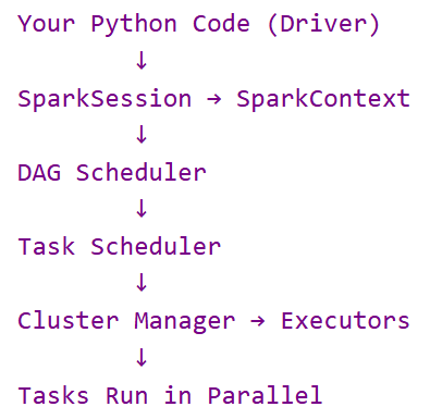
Understanding Spark architecture (Driver, Executors, Cluster Manager)
At its core, PySpark runs on top of the Apache Spark engine, which follows a master-slave architecture. Here's how the key components interact:
- Driver Program
This is your Python script or notebook.
It contains your SparkSession and defines the logic of your application.
It translates Python code into Spark jobs and coordinates execution.
- Cluster Manager
Allocates resources across the cluster.
Can be:
Standalone (built-in Spark manager)
YARN (Hadoop)
Mesos
Kubernetes
- Executors
These are worker processes launched on cluster nodes.
They execute tasks and store data in memory or disk.
Each executor runs multiple tasks in parallel.
- Tasks & Jobs
A job is triggered by an action.
Spark breaks the job into stages, and each stage into tasks.
Tasks are distributed to executors for parallel execution.
PySpark Flow Diagram (Conceptual)
RDD, DataFrame, and Dataset concepts
1. RDD (Resilient Distributed Dataset)
The RDD is the fundamental unit of data in Spark. It is a distributed collection of objects that are stored in memory or on disk across different nodes in a cluster.
Resilient: If a node fails, the RDD can rebuild itself using "lineage" (a log of transformations).
Distributed: Data is split into partitions across multiple nodes.
Dataset: It holds the data you're working with.
2. DataFrame
A DataFrame is a distributed collection of data organized into named columns. It is conceptually equivalent to a table in a relational database or a dataframe in R/Pandas, but with much richer optimizations under the hood.
Schema-based: Unlike RDDs, DataFrames have a schema (column names and types).
Optimized: DataFrames use the Catalyst Optimizer, which figures out the most efficient way to execute your query before it even starts.
3. Dataset
A Dataset is an extension of the DataFrame API that provides type-safety. It combines the "best of both worlds": the easy-to-use expressions of DataFrames and the strong typing of RDDs.
Type-Safe: In languages like Java or Scala, if you try to treat a "String" column like an "Integer," the code won't even compile.
Object-Oriented: You map your data to specific classes (Domain Objects)
Spark execution model (lazy evaluation, transformations, actions)
In Spark, nothing happens until it absolutely has to.
Lazy evaluation
means that data transformations are not executed immediately when defined.
Instead, Spark builds an optimized execution plan (a Directed Acyclic Graph, or DAG)
Actual computation is deferred until an action triggers the physical execution of the plan.
Transformations
Spark transformations are lazy operations that create a new DataFrame or RDD from an existing one, building a logical execution plan (DAG) without modifying the original data.
They only execute when an action is triggered

Actions
Actions return final values back to the driver's program.
They force the "lazy" transformations to actually run and compute results.
Any function that does not return to a new RDD is defined as an action.

SparkSession and SparkContext
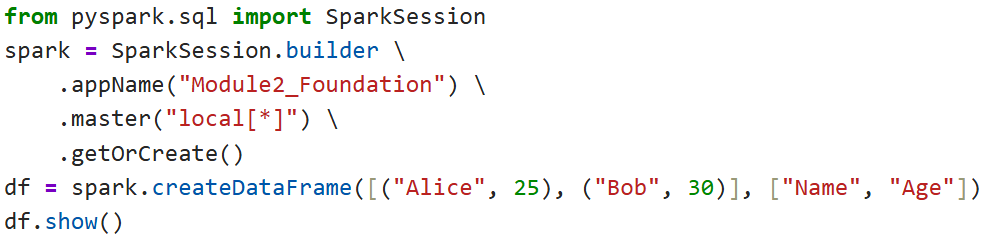
SparkSession: is the unified gateway to all Spark functionality. In older versions, you had to manage multiple contexts (SparkContext, SQLContext), but now one session handles everything.
Definition: A driver process that maintains the runtime environment and provides the entry point for Spark SQL and DataFrame APIs.
Example:
SparkContext :
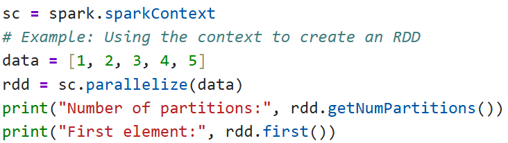
Definition: The low-level entry point for a Spark application that allows Spark to connect to a cluster. It is used primarily to create and manipulate RDDs (Resilient Distributed Datasets).
Example:
Relationship (How they work together):
Think of SparkSession as the controller, and SparkContext as one of its core engines:
SparkSession
├── SparkContext → RDDs, accumulators, broadcast variables
├── SQLContext → Spark SQL operations
├── HiveContext → Hive support
└── Config, Catalog, UDFs
2. Setting Up PySpark
Installing PySpark
For Mac / Linux
Install Java (Prerequisite): Spark requires a Java Virtual Machine (JVM) to run. Use Homebrew to install it easily: brew install openjdk@11
Install PySpark: The easiest method is using the Python package manager. This command downloads the Spark binaries automatically: pip install pyspark
Set Environment Variables: To let your terminal find Spark commands, add the following to your shell configuration file (like .zshrc or .bash_profile):

For Windows
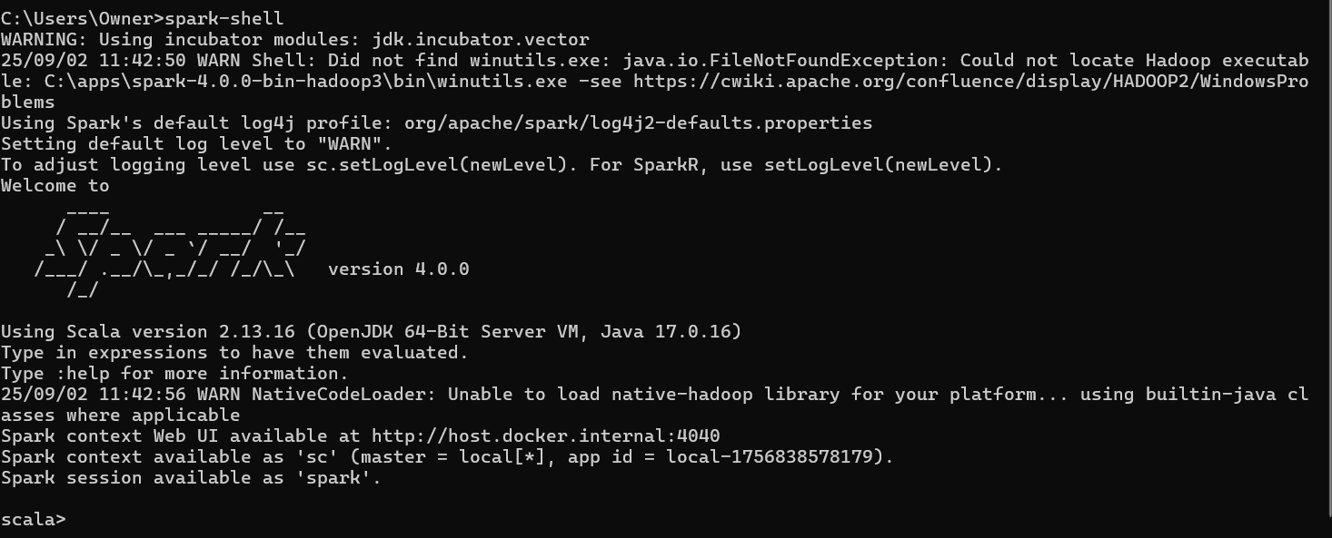
Download Spark & Java: Install Java (JDK 8 or 11) and Python. Then, download the Apache Spark .tgz file from the official site and unzip it to a folder (e.g., C:\Spark).
Winutils Setup (Critical): Windows needs a specific Hadoop binary to run Spark. Download winutils.exe for your Spark version and place it strictly in C:\Spark\bin.
Configure Variables: Go to "Edit System Environment Variables". Create SPARK_HOME pointing to C:\Spark, HADOOP_HOME pointing to C:\Spark, and add %SPARK_HOME%\bin to your system Path.
Creating SparkSession
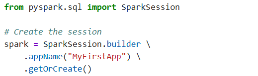
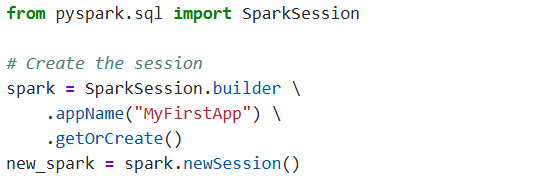
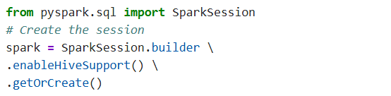
SparkSession serves as the unified entry point, utilizing a builder patterns to efficiently retrieve an active session or create a new one via getOrCreate().
builder.getOrCreate() Standard 99% of use cases (Production & Dev).
newSession() Isolation Multiple users/jobs in one app needing separate temporary views.
SparkSession(sc) Legacy Wrapping an old SparkContext (RDDs) into a DataFrame session.

enableHiveSupport() WarehouseConnecting to persistent Hive Metastores.
Configuration basics
Master URL: You must specify a master URL, such as .master("local"), to tell Spark to run on your laptop rather than a cluster.
Custom Configs: Use the .config() method to tweak settings, such as memory allocation or executor cores, before the app starts.
Web UI: Once configured and running, you can track your application's jobs and resource usage via the Spark Web UI (default: localhost:4040).

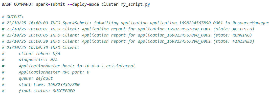
Local vs cluster mode
The Difference: The key distinction is where the "Driver" (the brain of your app) runs: on your machine (Client) or inside the cluster (Cluster).
Client Mode: Best for development and testing; if you close your laptop or terminal, the application stops immediately.
Cluster Mode: Best for production; the driver runs on a cluster node, so the job continues running even if you disconnect.
- Reading Data
Reading CSV files
Use the csv() method to load comma-separated data, ensuring you set header=True if the first row contains column names.

Reading JSON files
Use the json() method to read semi-structured data, which automatically handles the parsing of complex or nested data structures.

Reading Parquet files
Use the parquet() method to read this optimized, columnar storage format which preserves the original schema automatically.

Reading from databases (JDBC)
Use the jdbc format with connection properties (URL, user, password) to read tables directly from RDBMS like MySQL or PostgreSQL.

Schema inference vs explicit schema
Inference (inferSchema=True): Spark performs an extra pass over the data to automatically guess types (e.g., converting "123" to Integer), which is great for quick prototyping but slower for large files.

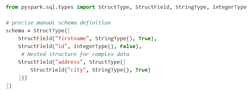
Explicit Schema: You manually define the structure upfront, which improves performance by skipping the inference scan and strictly enforces data consistency.
Core Components: A schema is defined using StructType (the table definition) which contains a list of StructField objects (individual columns).
Column Details: Each StructField specifies the column name, data type (e.g., StringType, IntegerType), and whether null values are allowed.
Complex Data: You can handle advanced data by nesting a StructType inside a field (parent-child relationship) or using ArrayType for lists.
Definition Styles: Schemas can be defined programmatically with objects or simply using DDL strings like "id INT, name STRING" for readability.
4. Basic DataFrame Operations
show(), printSchema(), describe()
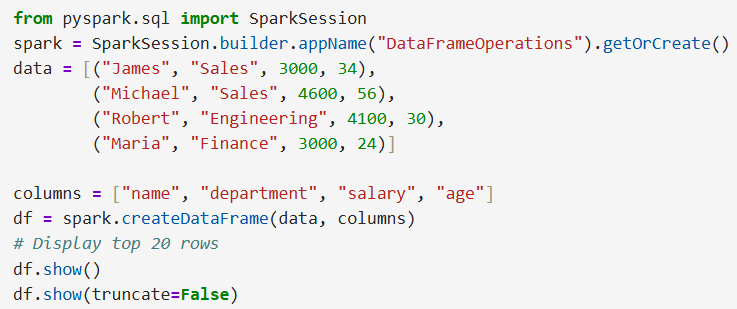
show(): Displays the top 20 rows of your DataFrame in a tabular format, automatically truncating long strings to keep the output clean.
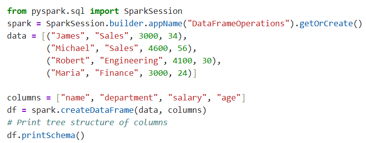
printSchema(): Prints the full structure of your DataFrame as a tree, revealing column names, data types (e.g., Integer, String), and nullability.
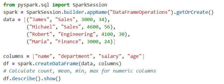
describe(): Calculates summary statistics for numeric columns, providing a quick view of count, mean, standard deviation, min, and max values.
select() and selectExpr()
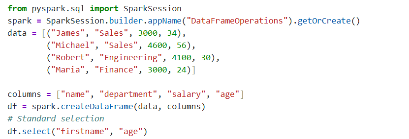
select(): Used to pick specific columns from your DataFrame to create a new one, similar to a standard SQL SELECT statement.
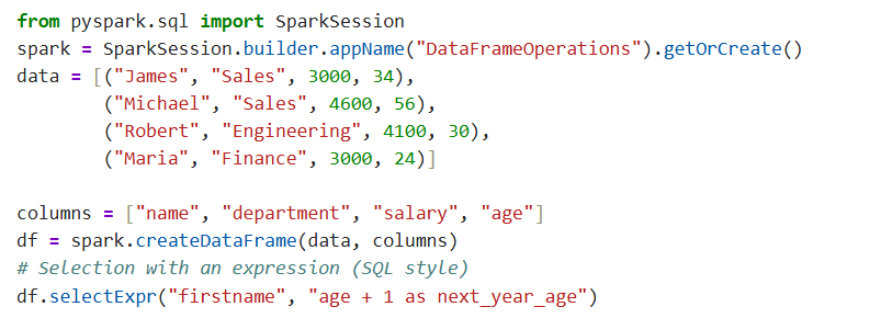
selectExpr(): A powerful variant that allows you to write SQL-style expressions directly (e.g., "age * 2") without needing extra functions.
filter() and where()
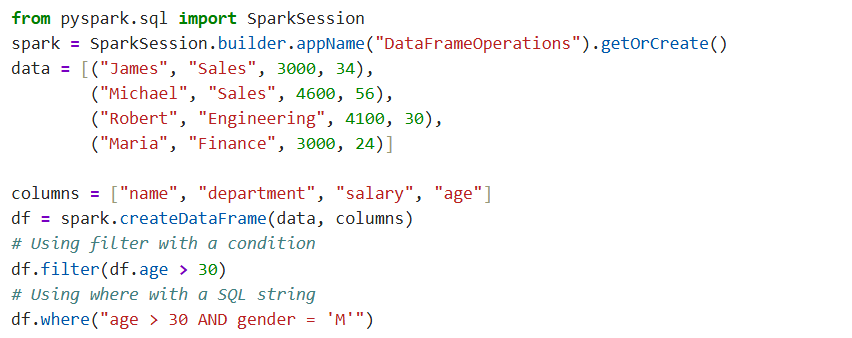
Synonyms: In PySpark, filter() and where() are identical; where() is simply an alias provided for those more comfortable with SQL syntax.
Conditioning: Both methods accept boolean conditions or SQL string expressions to return a new DataFrame containing only matching rows.
Chaining: You can easily chain multiple filters together (e.g., .filter(...).filter(...)) to narrow down your data step-by-step.
orderBy() and sort()
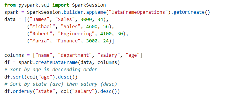
Identical Functionality: Like filter/where, orderBy() and sort() perform the exact same operation: sorting rows based on one or more columns.
Default Behavior: By default, both methods sort data in ascending order; you must explicitly use .desc() for descending order.
Multiple Columns: You can pass multiple column names to sort by a primary column first, then a secondary column if there are ties.
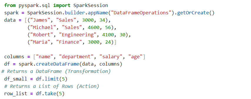
limit() and take()
Transformation vs. Action: limit(n) is a transformation that returns a new DataFrame with n rows, keeping the data distributed.
Driver Collection: take(n) is an action that returns a list of the first n Row objects directly to your driver (local machine).
Usage Rule: Use limit() when you want to continue processing data; use take() only when you need to inspect a small amount of data locally.
5. Column Operations
Adding columns (withColumn)
Creation & Update: The withColumn(name, expression) method creates a new column if the name doesn't exist, or replaces the column if it does.
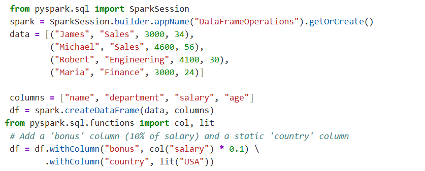
Row-wise Evaluation: It evaluates the provided expression for every single row in the DataFrame to generate the new values.
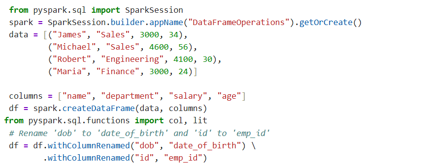
Renaming columns (withColumnRenamed)
Metadata Change: This operation changes the column's identifier in the schema without modifying the underlying data values.
Syntax: It takes two arguments: the existing_name and the new_name.
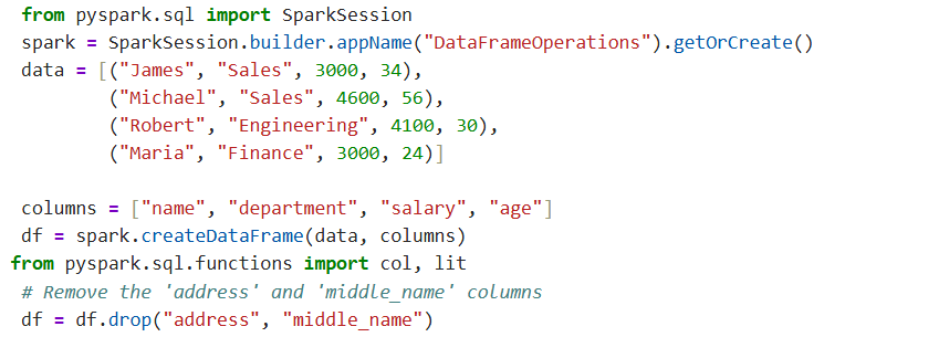
Dropping columns (drop)
Removal: The drop() method removes one or more columns from the DataFrame, returning a new DataFrame with the reduced schema.
Efficiency: This is a metadata-only operation and is very fast; it does not physically delete data from disk, just from the current DataFrame view.
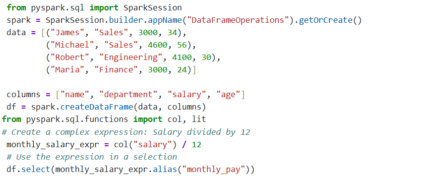
Column expressions
The Concept: A "Column Expression" is any operation applied to a generic Column object, such as arithmetic (col("age") + 1) or logic (col("age") > 18).
Programmatic Access: You construct these using the col() function or by accessing the DataFrame attribute (e.g., df.age).
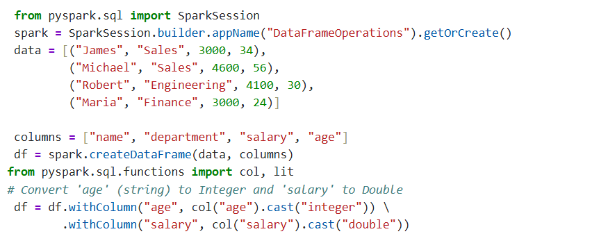
Casting data types
Type Conversion: The cast() method converts a column from one data type to another (e.g., String to Integer).
Data Cleaning: It is essential for fixing schema issues, such as when numbers are accidentally read as text strings.
Null Safety: If a value cannot be converted (e.g., casting "Hello" to Integer), Spark will safely return null instead of crashing.
6. Basic Aggregations
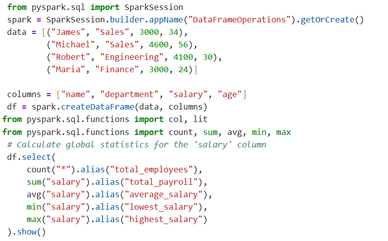
count(), sum(), avg(), min(), max()
Statistical Functions: These are standard SQL-like functions imported from pyspark.sql.functions to compute statistics on specific columns.
Global Aggregation: When used inside select(), they calculate the metric for the entire DataFrame (e.g., total revenue of the company).
Null Handling: Most aggregate functions automatically ignore null values during calculation (e.g., avg only counts rows with actual numbers).
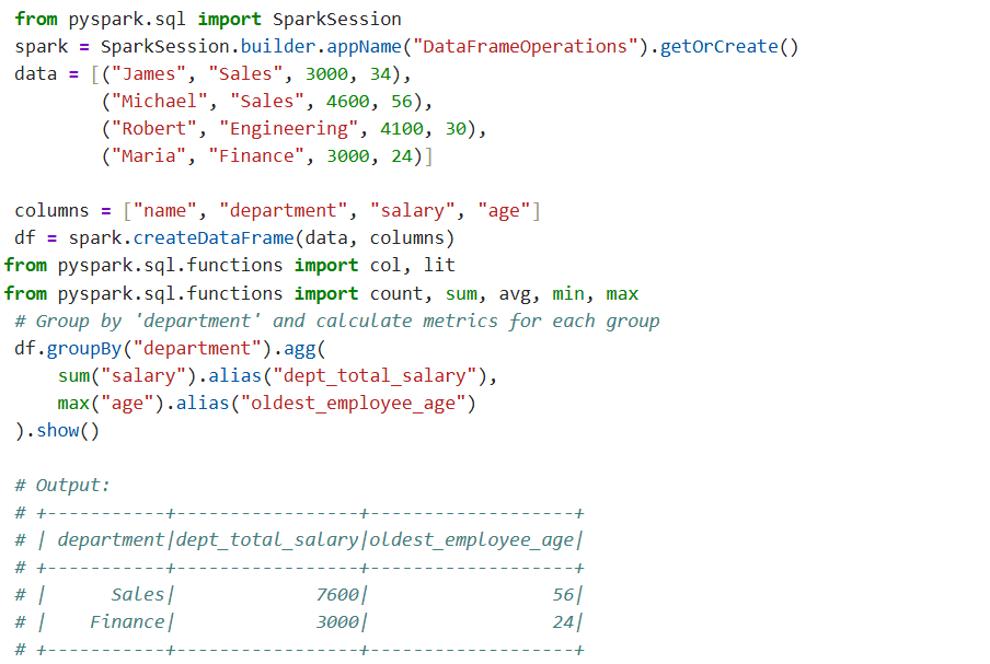
groupBy() and agg()
Grouping Data (groupBy): This transforms the DataFrame into a RelationalGroupedDataset by splitting rows into groups based on identical values in a specific column (e.g., grouping employees by "Department").
Multiple Aggregations (agg): The agg() method lets you apply different functions to different columns within those groups simultaneously (e.g., count employees AND average salary per department).
Result: The output is a new DataFrame where each row represents one unique group (e.g., one row per Department) with the calculated metrics.
7. Writing Data
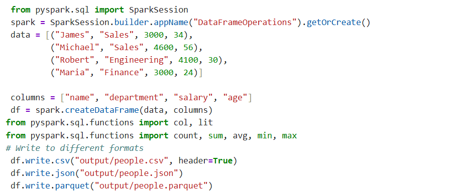
Writing CSV, JSON, Parquet
Unified API: The write property on a DataFrame provides access to the DataFrameWriter, which supports multiple formats (csv, json, parquet, etc.).
Format Selection: Use .csv("path"), .json("path"), or .parquet("path") to save your data.
Compression: Parquet is the default and recommended format because it compresses data efficiently and preserves schema information.
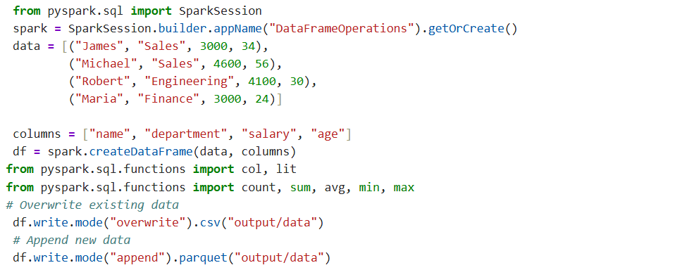
Write modes (overwrite, append, ignore, error)
Control Behavior: The mode() method determines what happens if the output directory already exists.
Overwrite: Completely deletes the existing directory and replaces it with the new data.
Append: Adds the new data files to the existing directory without deleting old ones.
Ignore: If the directory exists, the write operation is silently skipped (no error, no data written).
Error (Default): Throws an exception if the directory already exists to prevent accidental data loss.
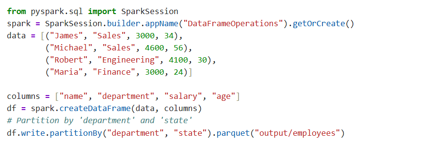
Partitioning output
Folder Structure: The partitionBy("column") method organizes output files into subdirectories based on column values (e.g., year=2023/month=01).
Performance: This dramatically improves read performance later because Spark can skip reading irrelevant partitions (directory pruning).
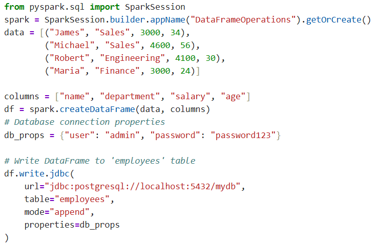
Writing to databases
JDBC Writer: Use the .jdbc() method to write DataFrame content directly into a relational database table.
Table Handling: The mode parameter is critical here; overwrite will drop and recreate the table, while append adds rows to the existing table.
Properties: You must provide the JDBC URL, target table name, and a properties dictionary containing credentials.
8. Basic SQL in Spark
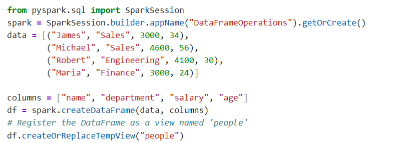
Creating temporary views
Bridge to SQL: The createOrReplaceTempView("view_name") method registers a DataFrame as a virtual table in memory, allowing you to query it using standard SQL syntax.
Session Scope: These views are temporary and exist only for the duration of your current SparkSession; they disappear when the session ends.
Replacement: If a view with the same name already exists, this method silently replaces it, which is useful for iterative development.
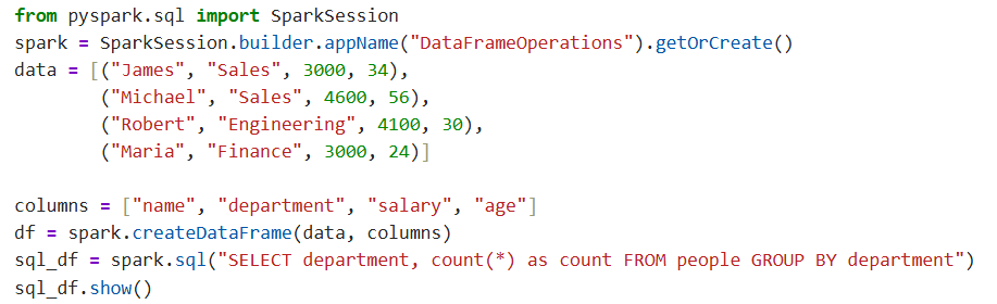
Running SQL queries with spark.sql()
Execution: The spark.sql("query_string") method allows you to execute standard SQL commands (SELECT, GROUP BY, WHERE) directly on registered views.
Return Type: The result of any SQL query is always a DataFrame, meaning you can immediately chain other PySpark operations (like .filter() or .show()) to the result.
Integration: You can seamlessly mix SQL and DataFrame code; for example, creating a DataFrame with SQL and then saving it with Python.
Pyspark Intermediate
1. Advanced DataFrame Operations
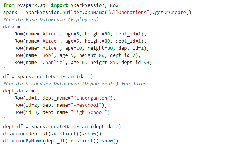
Union and unionByName
union() merges two DataFrames that have the exact same schema and column order, keeping all duplicates.

unionByName() is safer to use when columns are the same but in a different order, as it matches them by name.

To remove duplicate rows after a union, you must chain the distinct() method.
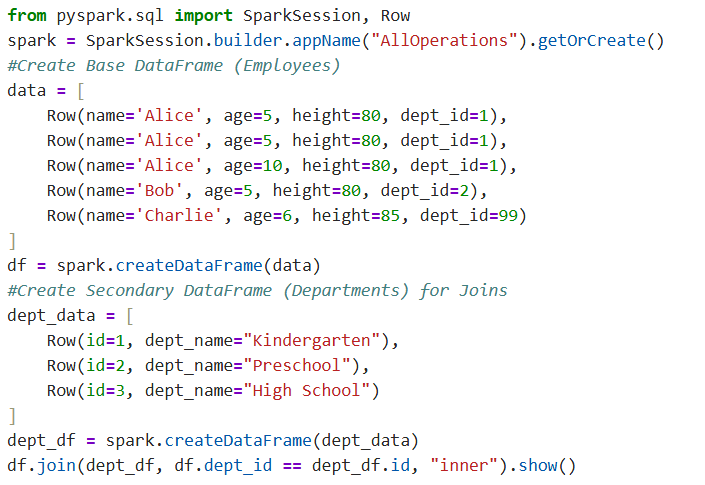
Join operations (inner, left, right, outer, cross, anti, semi)
The join() method combines two DataFrames based on a shared column or condition.
You can specify types like "inner" (matches only), "left" (all left rows), or "outer" (all rows from both), anti(dataframe but not in other).
If no type is specified, PySpark defaults to an "inner" join.
Inner Join: Returns only the rows where there is a match is found
Left (Outer) Join: Returns all rows of the Left Dataframe with or without match

Right (Outer) Join: Returns all rows of the Right Dataframe with or without match

Full (Outer) Join: Returns all rows of the Both Dataframe with or without match

Left Semi Join: Returns only rows from the Left DataFrame that have a match in the right DataFrame.

Left Anti Join: Returns only rows from the Left DataFrame that do not have a match on the right.

Cross Join: Combines every single row from the left DataFrame with every single row from the right (Cartesian product).

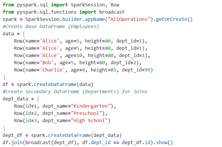
Broadcast joins
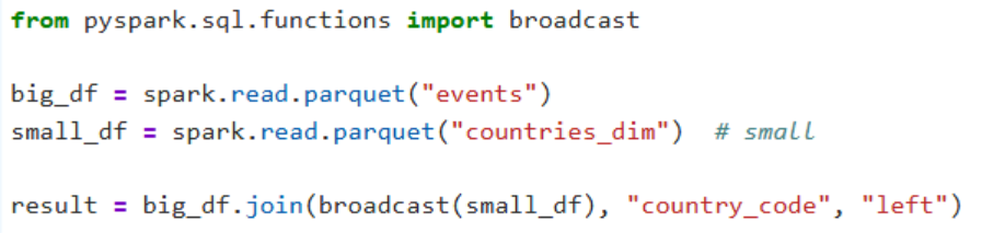
This is a performance optimization used when joining a large DataFrame with a very small one.
It sends a copy of the small table to every worker node, avoiding expensive data shuffling across the network.
You simply wrap the smaller DataFrame with the broadcast() function to trigger this.
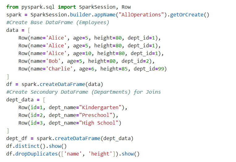
Duplicate handling (distinct, dropDuplicates)
distinct() checks every single column in a row and removes exact duplicates.
dropDuplicates() is more flexible, allowing you to remove duplicates based only on specific columns.
Both operations return a new DataFrame with unique records, leaving the original unchanged.
2. Built-in Functions
String functions (concat, substring, regexp_replace)
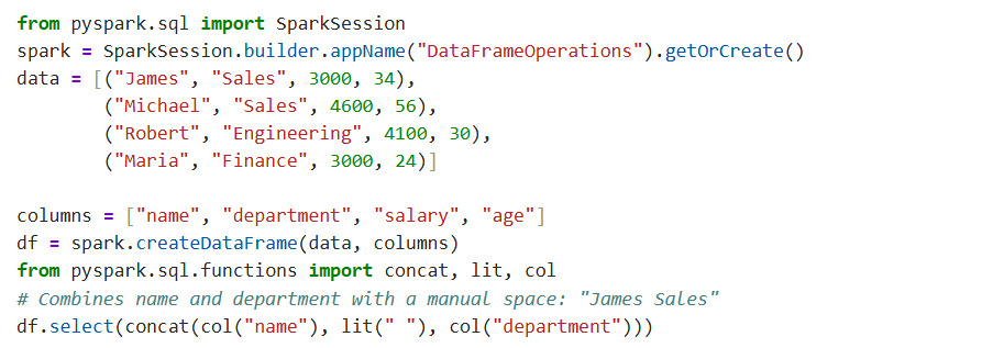
concat():
merges the values of multiple columns or literal strings into one continuous string without any separators.
Use concat_ws(separator, cols) if you want to add a separator (like a space or comma) between them automatically.
substring():
slices a string starting from a specific index (pos) and grabs a set number of characters (len).

regexp_replace():
uses patterns (regular expressions) to find and replace text within a string.

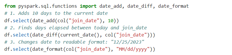
Date and time functions (date_add, date_diff, date_format)
date_add() creates a new date by adding a specified number of days to an existing date column.
date_diff() calculates the difference in days between two dates.
date_format() converts a standard date object into a custom string format (like "MM-dd-yyyy").
Mathematical functions
Arithmetic Operator: Basic math operators (+, -, *, /) work directly on column objects to perform element-wise calculations.
Syntax: col("a") + col("b") | col("a") - col("b") | col("a") * col("b") | col("a") / col("b")

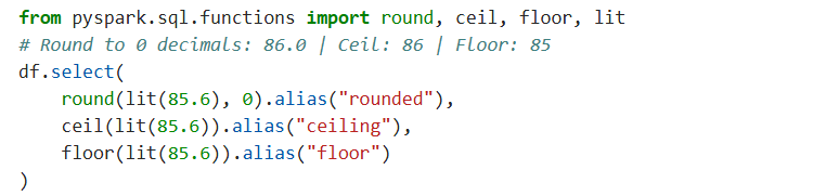
Rounding Functions:
round(): Nearest integer
ceil(): Next Whole integer
floor(): Previous Whole integer
Syntax: round(col, scale) | ceil(col) | floor(col)
Root Functions: sqrt() calculates the square root of a numerical column.
Syntax: sqrt(col)

Trigonometric Functions: Functions like sin(), cos(), and tan() calculate the sine, cosine, and tangent of a value
Syntax: sin(col) | cos(col) | tan(col)

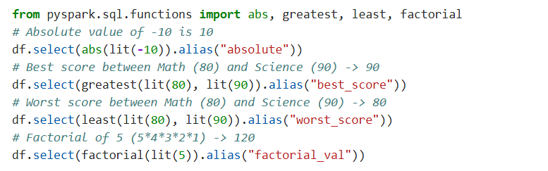
General Math Functions:
abs():return absolute positive value
greatest() and least(): compare multiple columns row-by-row to find the highest or lowest value among them.
factorial(): computes the product of all positive integers up to that number (e.g., 4! = 24).
Syntax: abs(col) | greatest(col1, col2, ...) | least(col1, col2, ...) | factorial(col)
Collection functions (array, map operations)
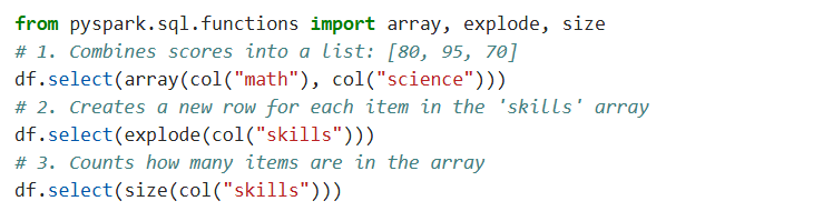
array() creates a list (collection) of data from multiple columns in a single row.
explode() is a powerful function that splits an array into separate rows (one row per item).
size() returns the number of elements contained in an array or map
Conditional functions (when, otherwise)
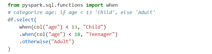
when() checks a condition and returns a value if true (similar to an "if" statement).
otherwise() defines the fallback value if the condition is false (similar to "else").
You can chain multiple .when() calls together to handle complex logic.
3. Handling Missing Data
Detecting null values
Identification: use the isNull() method on a specific column to find rows where data is missing or undefined.
Filtering: commonly used inside a filter() or where() clause to isolate incomplete records for inspection.
Counting: chaining this with count() helps you quantify exactly how many missing values exist in your dataset.

Dropping nulls (na.drop)
na.drop() (or dropna()) method removes rows containing any null values, ensuring a clean dataset.
how="all" to drop rows only if all columns are null.
subset=["col_name"] you can pass a list of column names

Filling nulls (na.fill)
Smart Substitution: The na.fill() method replaces nulls with constants, automatically applying values only to matching data types (e.g., 0 for integers, "Unknown" for strings).
Precision: You can also pass a dictionary {"col_name": value} to target specific columns with different default values simultaneously.

Replacing values (na.replace)
Targeted Swapping: The na.replace() method finds and replaces specific existing values (not just nulls) across the entire DataFrame or selected columns.
Efficient Mapping: You can use a simple dictionary (e.g., {"": None}) to map old values to new ones, perfect for cleaning standard data errors.

Custom null handling strategies
Conditional Logic: for complex rules (e.g., "if age is null, set it to the average"), use the when().otherwise() functions.
Precision: this strategy allows you to calculate dynamic defaults based on other column values rather than using a static constant.

4. Window Functions
Window specifications
Definition: A Window Specification defines the specific "frame" or group of rows that a function will operate on, without collapsing the data like a standard GROUP BY.
Creation: You use the Window utility class to build these specifications, acting as a blueprint for your calculations.
Components: It typically combines partitioning (grouping) and ordering (sorting) to tell Spark exactly which rows relate to the current row.

Partitioning and ordering
Partitioning: The partitionBy() method splits your data into distinct groups (e.g., Departments), ensuring calculations restart for each group.
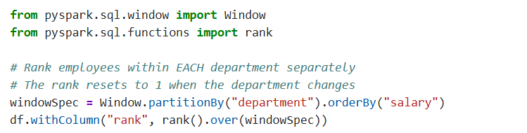
Ordering: The orderBy() method arranges the rows within those partitions (e.g., lowest to highest salary), which is critical for ranking or running totals.

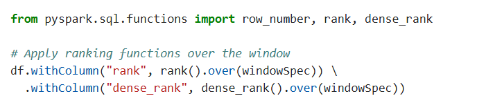
Ranking functions (row_number, rank, dense_rank)
Row Number: row_number() assigns a unique, sequential integer to every row, even if values are identical (1, 2, 3, 4).
Rank: rank() assigns the same rank to ties but leaves gaps in the sequence (1, 2, 2, 4).
Dense Rank: dense_rank() assigns the same rank to ties without leaving gaps (1, 2, 2, 3).
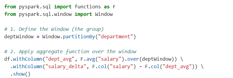
Aggregate window functions
Row-Level Aggregates: Unlike groupBy(), window aggregates append results (like avg or sum) to every individual row without collapsing the dataset.
Direct Application: You apply standard functions (avg, sum, max, min) directly over a WindowSpec to calculate values within a specific group or "frame."
LAG and LEAD
Looking Back/Forward: lag() retrieves data from a previous row, while lead() fetches data from a subsequent row within the partition.
Offsets: You can specify how many rows to look back/forward (default is 1) and providing a default value if that row doesn't exist (like 0 or null).

Cumulative operations
Running Totals: By adding rowsBetween (or rangeBetween) to your window, you can define a growing frame that calculates cumulative sums or moving averages.
Frame Definition: Window.unboundedPreceding creates a frame that starts at the very first row of the partition and extends to the current row.

5. User Defined Functions (UDFs)
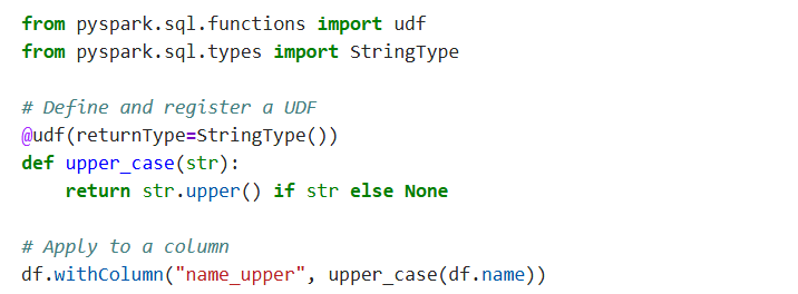
Creating Python UDFs
Create a standard Python function that performs your custom logic.

Registering UDFs
Custom Logic: UDFs allow you to write custom Python functions to perform complex transformations that are not available in the built-in Spark SQL functions.
Decoration: Use the @udf decorator or the udf() function to wrap a standard Python function, making it compatible with Spark DataFrames.
SQL Registration: If you want to use the function inside spark.sql() queries, you must also register it using spark.udf.register().
UDF return types
Type Definition: You must explicitly specify the returnType (e.g., IntegerType(), ArrayType()) so Spark knows how to handle the data coming out of Python.
Default Behavior: If no return type is specified, Spark defaults to StringType(), which may cause errors if your function returns numbers or complex objects.
Matching Schema: The Python object returned by your function must strictly match the Spark DataType defined in the registration.

Performance considerations
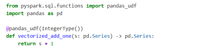
The "Serialization Tax": Python UDFs are significantly slower than built-in functions because Spark must move data from the JVM to a Python process and back (serialization).
Optimization (Pandas UDFs): For better performance, use Pandas UDFs (Vectorized UDFs), which use Apache Arrow to transfer data in batches rather than row-by-row.
Best Practice: Always check if a built-in Spark function (like upper() or when()) can do the job before resorting to a Python UDF, as built-ins run natively in the JVM.
6. Data Processing Patterns
Filtering and sampling
Filtering: Use the filter() (or where()) method to keep only the rows that match a specific condition, effectively removing irrelevant data.
Sampling: The sample() method extracts a random fraction of the dataset (e.g., 10%), which is perfect for testing code on large datasets without waiting for full processing.

Deduplication strategies
Removing Duplicates: The dropDuplicates() method removes rows that are identical across all columns or specific subsets of columns.
Key-Based: By passing column names (e.g., ["id"]), you ensure uniqueness based on those specific keys, keeping only the first occurrence found.

Data validation
Quality Checks: Validation involves ensuring data meets expectations (e.g., no nulls, correct formats) before processing, often using filter() or when() conditions.
Constraint Enforcement: You can flag or filter out records that violate business rules, such as ensuring an email column actually contains an "@" symbol.

Error handling
Graceful Failure: Instead of letting bad data crash your job, use conditional logic (when/otherwise) to tag rows as "Valid" or "Error".
Quarantine Pattern: Split your data into two streams: one for clean data to process and another for "bad records" to save for later analysis.

7. Caching and Persistence
cache() and persist()
Optimization: The cache() method is a shorthand that stores the DataFrame in Memory only, making subsequent actions on it much faster.
Flexibility: The persist() method does the same but allows you to choose where to store the data (e.g., Memory, Disk, or both) for better resource management.

Storage levels
Memory vs. Disk Trade-off: MEMORY_ONLY is the fastest but consumes the most RAM; if memory fills up, partitions are dropped and recomputed later. In contrast, MEMORY_AND_DISK (the DataFrame default) spills excess data to disk, preventing recomputation at the cost of slower I/O speed.
Serialization Efficiency: Levels with _SER (like MEMORY_ONLY_SER) store data as serialized byte arrays, which drastically reduces memory usage (space-efficient) but increases CPU load because the data must be deserialized every time it is read.
Fault Tolerance via Replication: Any storage level ending in _2 (e.g., MEMORY_AND_DISK_2) replicates each partition on two different cluster nodes, ensuring that if one node fails, the data is instantly available from the other without needing recomputation.
unpersist()
Cleanup: The unpersist() method removes the DataFrame from memory or disk, freeing up resources for other tasks.
Blocking: By default, this happens asynchronously, but you can pass blocking=True to wait until the memory is fully cleared before proceeding.

When to cache
Iterative Reuse: Caching is mandatory for iterative algorithms (like Machine Learning loops or Graph processing) where the same dataset is accessed repeatedly, preventing Spark from re-calculating the entire lineage 100 times.
Multiple Actions: If you plan to trigger multiple distinct actions (e.g., count() then write()) on the same transformed DataFrame, caching ensures the transformations run only once instead of re-executing from scratch for every action.
Expensive Upstream: Always cache a DataFrame that results from "heavy" operations (like complex joins or massive aggregations) so subsequent steps don't have to pay the high computational cost of those joins again.

8. Basic RDD Operations
Creating RDDs
Parallelize: The simplest way to create an RDD is by using spark.sparkContext.parallelize() on an existing Python list or collection.

External Data: You can also create RDDs by reading external storage, such as text files, using spark.sparkContext.textFile("path/to/file.txt").

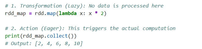
Lazy Evaluation: Remember, creating an RDD defines a lineage but does not load data into memory until an action (like collect) is called.
Map, filter, flatMap
Map: A 1-to-1 transformation that applies a function to each element, returning exactly one output element for every input element.

Filter: A selection operation that returns a new RDD containing only the elements that satisfy a specific condition (boolean true).
FlatMap: A 1-to-many transformation that flattens results; if your function returns a list (like splitting a line into words), flatMap merges them into a single list.

Reduce, reduceByKey
Reduce: An action that aggregates all elements of the RDD using a specified commutative and associative operator (like addition) to return a single result to the driver.
ReduceByKey: A transformation used on Pair RDDs (key-value pairs) to aggregate values for each key separately, which is efficient because it performs local aggregation before shuffling.
Efficiency: reduceByKey is preferred over groupByKey for aggregations because it reduces data traffic across the network significantly.
Converting between RDD and DataFrame
To DataFrame: Use the toDF() method on an RDD of tuples or spark.createDataFrame(rdd) to convert unstructured RDD data into a structured DataFrame with a schema.
To RDD: You can convert a DataFrame back to an RDD of Row objects simply by accessing the .rdd attribute.
Interoperability: This allows you to switch between low-level functional programming (RDDs) and high-level optimized SQL queries (DataFrames) as needed.
Pyspark Advance
1. Performance Optimization
Understanding Spark UI and execution plans
Spark UI
Web interface to monitor your Spark application (jobs, stages, tasks).
Helps you find bottlenecks: slow stages, skewed tasks, heavy shuffles.
Key views
Jobs: list of actions triggered, their status and duration.
Stages: Shows shuffle vs non-shuffle stages, input/shuffle size, time taken.
Tasks: per-task metrics (run time, GC time, errors, skewed tasks).
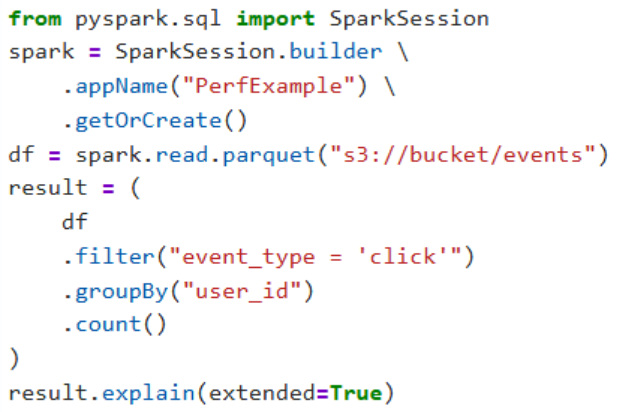
Execution plan from code
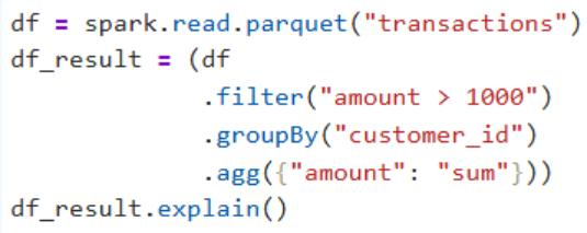
Use explain to see logical and physical plans for a DataFrame.
Catalyst optimizer
Concept
Core optimizer for Spark SQL/DataFrame queries.
Converts your code into an optimized logical and physical plan before execution.
What it does
Predicate pushdown: moves filters closer to the data source.
Column pruning: reads only required columns.
Constant folding and simple expression simplification.
Chooses join order and join types based on estimated sizes.
How you “help” it
Filter early, select only needed columns.
Prefer built-in functions and DataFrame/SQL APIs over Python UDFs.
Tungsten execution engine
Concept
Low-level engine that executes the physical plan produced by Catalyst.
Focuses on CPU efficiency and memory management.
Key ideas
Whole-stage code generation (JVM bytecode for pipelines of operators).
Compact binary format in memory to reduce GC overhead.
Cache-friendly, vectorized processing.
Impact
DataFrame/SQL operations are usually faster than equivalent RDD code.
Complex expressions using built-in functions benefit the most.
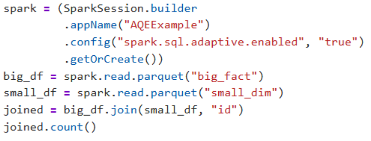
Adaptive Query Execution (AQE)
Concept
Lets Spark adjust the physical plan at runtime using real data statistics.
Main features
Dynamic join selection: convert shuffle join to broadcast join if one side is small.
Coalescing shuffle partitions: merge many tiny partitions into fewer larger ones.
Basic skew handling for heavily skewed partitions.
Usage
Enabled via configuration, visible in final physical plan and Spark UI.
Partitioning strategies
Concept
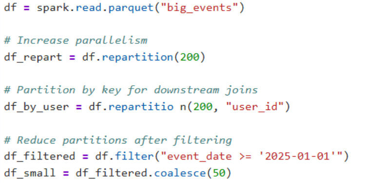
Controls how data is split into partitions across executors.
Affects parallelism, skew, and shuffle cost.
Goals
Enough partitions to use the cluster well, but not too many tiny tasks.
Partitions of similar size to avoid skew.
Align partitioning with common join/groupBy keys where possible.
APIs
repartition(n): full shuffle, evenly distribute into n partitions.
repartition(n, "col"): hash-partition by a key column.
coalesce(n): reduce partitions with minimal shuffle.
Shuffling optimization
Concept
Shuffle = data redistributing across nodes (network + disk I/O).
Triggered by wide transformations like join, groupBy, distinct, orderBy.
Why optimize
Shuffles often dominate job runtime and resource usage.
Techniques
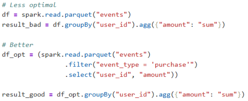
Filter early to reduce rows before a shuffle.
Select only necessary columns before join/groupBy.
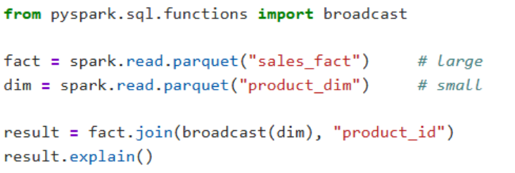
Use broadcast joins when one side is small.
Tune spark.sql.shuffle.partitions to a reasonable value.
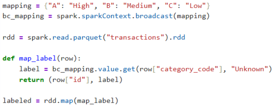
Broadcast variables
Concept
Small read-only data sent once to each executor and reused by tasks.
Use cases
Broadcast joins: small dimension + large fact table.
Static mappings or configuration used in transformations.
Benefits
Avoids repeatedly shipping the same small data with each task.
Reduces shuffle when using broadcast joins.
DataFrame example:
RDD example:
Accumulators
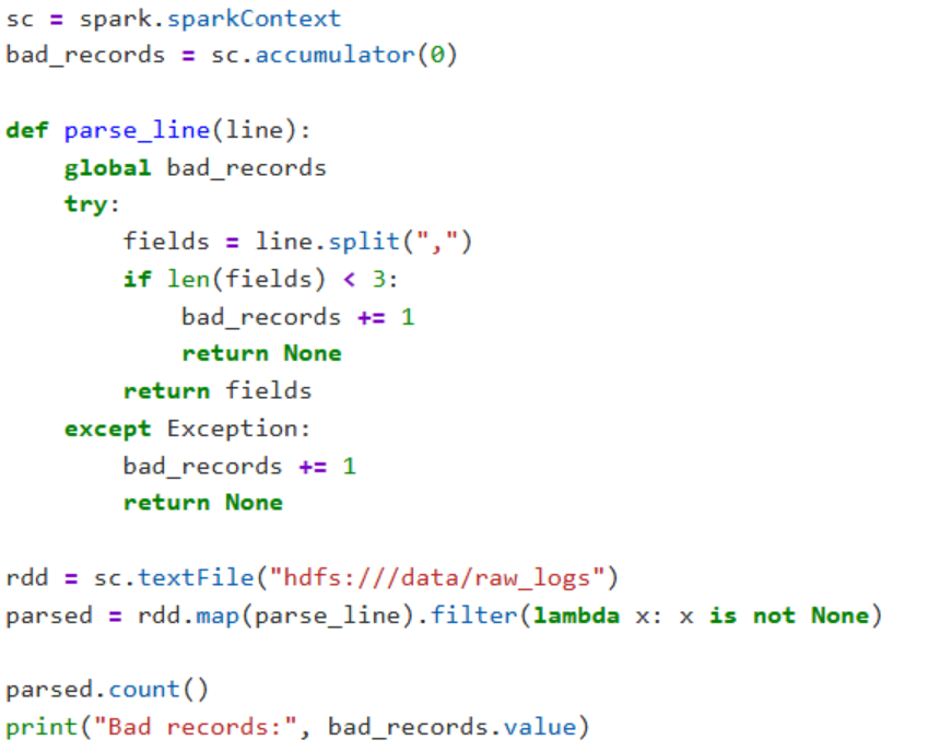
Concept
Variables that executors can add to and the driver can read as global counters.
Characteristics
Write-only from tasks, read on the driver.
Used for metrics/monitoring (e.g., bad row counts), not business logic.
2. Advanced Joins and Aggregations
Join optimization techniques
Prefer DataFrame/SQL joins over RDD joins for better optimization and performance.
Reduce data size before joins using filter and select to limit rows and columns.
Use broadcast joins when one table is small enough to fit in executor memory.
Choose appropriate join types (inner, left, semi, anti) to avoid unnecessary data.
Example (broadcast join):
Skewed join handling
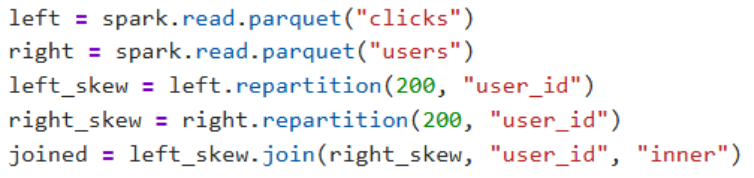
Skew happens when a few keys have a very large number of rows compared to others.
Symptoms: one or few tasks in a join stage run much longer than the rest.
Basic techniques:
Filter irrelevant data before join.
Repartition on join key to spread data more evenly.
Example (repartition on join key):
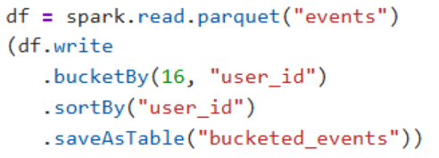
Bucketing
Bucketing groups data into a fixed number of buckets based on a column’s hash.
Buckets are stored as separate files but with consistent hash partitioning.
Benefits:
Efficient joins when both tables are bucketed on the same column and number of buckets.
Reduces shuffle for joins and aggregations on bucketed keys.
Example (creating a bucketed table):
Salting techniques
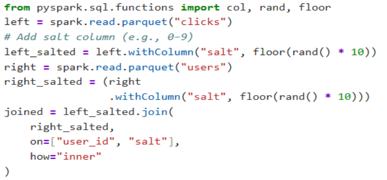
Salting is used to handle skewed keys by spreading them across multiple buckets.
Idea: add a random or calculated “salt” column for heavy keys before join.
Steps:
Duplicate rows for skewed keys with different salt values.
Join on both original key and salt to distribute load.
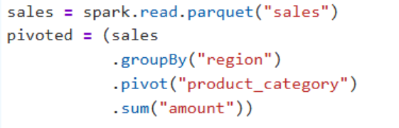
Advanced aggregation with pivot
Pivot converts unique values from one column into multiple columns.
Useful for reshaping data (e.g., metrics by category as columns).
Syntax: groupBy(...).pivot(pivot_col[, values]).agg(...).
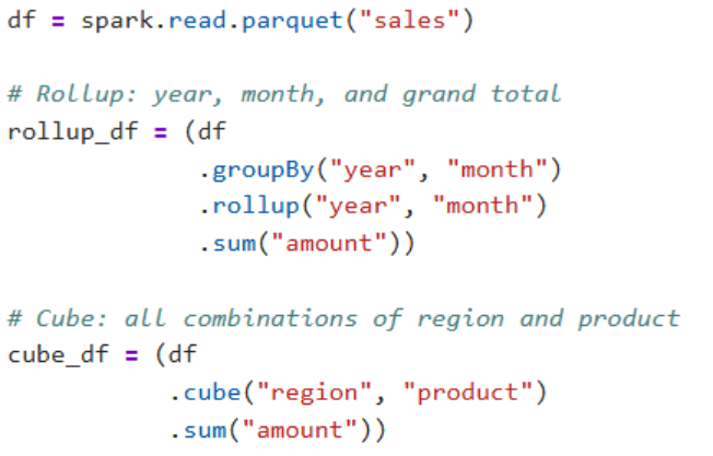
Cube and rollup operations
rollup
Creates subtotals along a hierarchy (e.g., year → month → day).
Produces grouped totals and grand total.
cube
Creates subtotals for all combinations of grouping columns.
Useful for multi-dimensional reports (e.g., by region, product, channel).
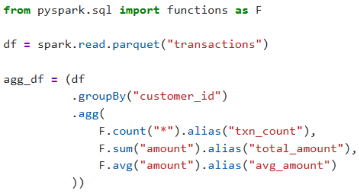
Multiple aggregations in single pass
Use a single groupBy with multiple aggregations to avoid repeated scans/shuffles.
Use agg with multiple expressions or agg with a dictionary
3. Spark SQL Advanced
Global and temporary views
Temporary views
Session-scoped; available only in the current SparkSession.
Useful for ad-hoc SQL on DataFrames without persisting metadata.

Global temporary views
Shared across all sessions in the same application, under the global_temp database.
Survive multiple SparkSessions as long as the application is running.

Catalog operations
Inspecting databases and tables
spark.catalog.listDatabases() to see available databases.
spark.catalog.listTables("db_name") to list tables in a database.
Inspecting columns and functions
spark.catalog.listColumns("table_name") to see schema info.
spark.catalog.listFunctions() to list registered functions (built-in + UDFs).
Dropping and refreshing
spark.catalog.dropTempView("view_name") to remove a temp view.
spark.catalog.refreshTable("table_name") to refresh metadata after external changes.
Database and table management
Database operations
Create database:

Use/change database:

Table operations
Create managed table from DataFrame:

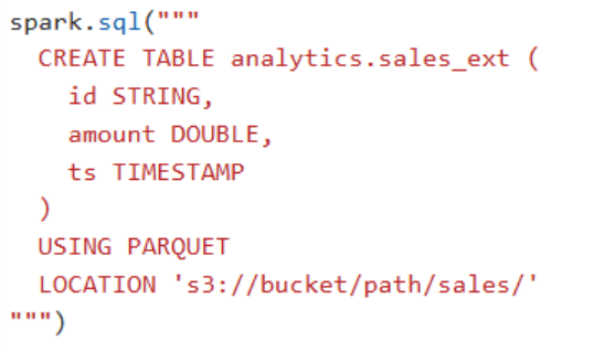
Create external table via SQL:
Alter and drop table:

SQL query optimization
Prefer SQL/DataFrame APIs over RDDs for automatic optimization.
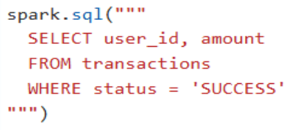
Push filters and projections down in SQL where possible.
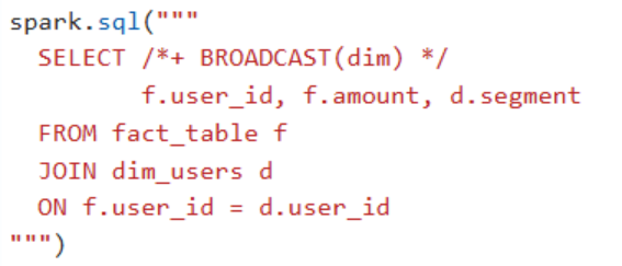
Use appropriate join hints when needed (e.g., broadcast hint).
Avoid unnecessary SELECT * in large tables; explicitly list needed columns.
Check execution plans using:

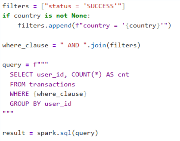
Dynamic SQL generation
Build SQL strings programmatically in Python based on parameters or conditions.
Useful for reusable queries, parameter-driven reports, or optional filters.
Simple example with string formatting:
4. Partitioning and Bucketing
Repartition vs coalesce
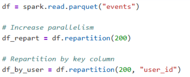
repartition
Changes the number of partitions by doing a full shuffle.
Good for increasing parallelism or redistributing data more evenly.
Can also repartition by a column (hash partition).
coalesce
Reduces the number of partitions with minimal or no shuffle.
Good after heavy filtering when many partitions are almost empty.
Typically used to reduce output files.

Custom partitioning
Concept
Manually controlling how data is partitioned (not only how many partitions).
Helpful when you know which key will be used for joins/aggregations.
Hash partitioning by column
Use repartition(num, "col") to hash-partition by a key.
Aligns future joins/groupBy operations on that column.

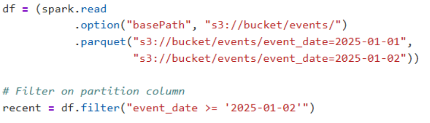
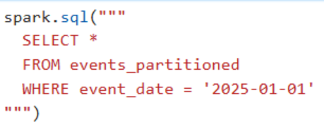
Partition pruning
Concept
Spark skips reading partitions that are not needed based on filter conditions.
Works when data is physically partitioned by a column (e.g., event_date).
With partition pruning, only the relevant event_date partitions are read.
Benefits
Reduces I/O and speeds up queries by avoiding irrelevant data.
Example (reading partitioned data):
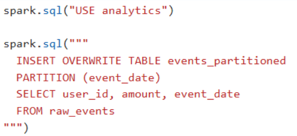
SQL/Hive-style partitioned table example:
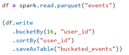
Bucketing for joins
Concept
Bucketing writes data into a fixed number of buckets based on the hash of a column.
Both tables bucketed on the same column and number of buckets can join more efficiently.
Benefits
Reduces shuffle when joining bucketed tables on the bucket column.
Useful for repeated joins between large tables on the same key.
Creating a bucketed table from a DataFrame:
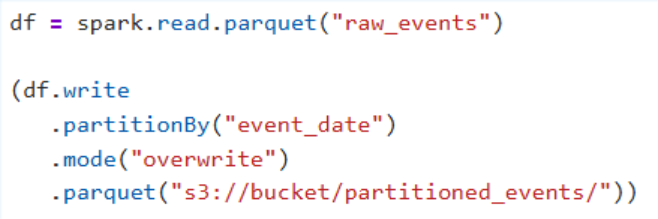
Dynamic partitioning
Concept
Partitions are created dynamically at write time based on column values.
Common with Hive-style partitioned tables and ETL pipelines.
When combined with partition pruning, dynamic partitioning makes downstream queries faster by organizing data by common filter keys.
Writing dynamically partitioned data (DataFrame API):
Writing into a partitioned table with Spark SQL:
5. Memory Management
Memory configuration
Concept
Spark divides cluster resources into driver and executor processes.
Each executor has its own memory, split between execution (for shuffles, joins, aggregations) and storage (for caching/persisting data).
Key settings (high level, not tied to any one cluster manager):
Executor memory: controls how much memory each executor gets for data and computation.
Executor cores: number of parallel tasks an executor can run; affects how memory is shared between tasks.
Overhead/reserved memory: extra memory kept aside for JVM overhead, metadata, and non-data structures.
Executor vs driver memory
Driver memory
Belongs to the process that runs your PySpark application (your script or notebook).
Stores:
SparkSession, SparkContext, query plans, job metadata.
Collected results when you use actions like collect() or toPandas().
Risks:
Using collect() or toPandas() on very large DataFrames can exhaust driver memory and crash the application.
Guidelines:
Use driver memory mainly for control/coordination and small result sets.
For large data, write to storage (files, tables) instead of collecting everything to the driver.
Executor memory
Belongs to worker processes that run tasks on partitions of your data.
Used for:
Holding partitions in memory during transformations and actions.
Performing joins, aggregations, and shuffles (execution memory).
Storing cached/persisted RDDs/DataFrames (storage memory).
Behavior:
When execution memory is not enough, Spark spills intermediate data to disk.
When storage memory is tight, cached blocks may be evicted to make room.
Guidelines:
Allocate enough memory per executor so that typical joins/aggregations do not spill excessively.
If you cache data heavily, ensure storage memory is sufficient and selectively unpersist unused data.
6. Testing and Debugging
Unit testing Spark applications
Concept
Validate individual transformation functions using small, in-memory DataFrames.
Use Python testing frameworks like unittest or pytest with a local SparkSession.
Typical pattern
Create a SparkSession once for the test suite.
Build small input DataFrames with spark.createDataFrame.
Apply your transformation function.
Compare the result to an expected DataFrame (schema + data).
Integration testing
Concept
Test full pipeline behavior, including reading from/writing to storage.
Closer to real production runs (I/O, configs, multiple stages).
Typical pattern
Use a test cluster or local mode with realistic configs.
Prepare small input files in a test path (e.g., local FS, temp directory).
Run your job (or main ETL function) end-to-end.
Validate outputs by reading result tables/files and asserting on content.
Debugging strategies
Use Spark UI
Inspect slow jobs/stages, look at task durations, shuffle read/write sizes.
Look for skew: a few tasks taking much longer than others in the same stage.
Narrow down transformations
Add intermediate .limit() + show() or head() at critical points to inspect data.
Keep transformations small and composable so they are easier to test and debug individually.
Check execution plans
Use df.explain(True) and spark.sql("EXPLAIN EXTENDED ...") to see join types, shuffles, and filters.
Local vs cluster
Reproduce issues in local mode with reduced data when possible.
For cluster-only issues, rely on Spark UI, logs, and metrics.
Logging best practices
Use standard logging libraries (e.g., Python logging) instead of print.
Include key information in log messages: input sizes, filter conditions, important IDs, and counts.
Set appropriate log levels
INFO for normal pipeline progress (start/end of stages, record counts).
WARN/ERROR for data issues, exceptions, or retries.
Avoid logging entire rows or huge DataFrames; log summaries (counts, sample IDs).
Configure log level per environment (more detailed in dev, less in prod).
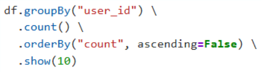
Handling data skew
Detecting skew
In Spark UI: a few tasks in a stage much slower than others, with very high input or shuffle read.
In code: df.groupBy("join_key").count().orderBy("count", ascending=False).show() to see “heavy” keys.
Mitigation techniques
Filter out unnecessary data before joins/aggregations.
Repartition by the join/group key to spread data more evenly.
Use salting: add an extra random or calculated key for hot keys to distribute them across partitions.
Process very hot keys separately and union their results with the rest.
7. Data Quality and Validation
Schema evolution
Concept
Schema changes over time (new columns, removed columns, type changes) are common in real pipelines.
Poorly managed schema evolution can break jobs or silently corrupt data quality.
Typical scenarios
Adding new optional columns to existing datasets or tables.
Merging data from multiple sources with slightly different schemas.
Evolving data types in a compatible way (for example, int to long).
Strategies in PySpark
Use schema-on-read (define schemas in code when reading) instead of relying only on inferred schemas.
For formats like Delta/Parquet, enable controlled schema merge options when needed (for example, mergeSchema for Delta).
Add data quality checks around schema changes to ensure new columns or types behave as expected.
Data validation frameworks
Purpose
Automate checks on Spark DataFrames: nulls, ranges, uniqueness, row counts, patterns, and custom business rules.
Integrate data quality into pipelines instead of manual, ad-hoc checks.
Common tools (Spark/PySpark friendly)
Great Expectations: works directly with Spark DataFrames; lets you define “expectations” and generate validation reports.
Deequ / PyDeequ: Spark-based library for declarative constraints and metrics over large datasets.
Spark-specific libraries like Drunken Data Quality / DDQ (constraint checks on Spark data structures).
Typical checks
Schema validation (column presence, data types).
Null checks, value ranges, allowed value lists.
Uniqueness and primary-key-like constraints.
Constraint enforcement
Concept
Express explicit rules that your data must satisfy and fail/alert when they don’t.
Types of constraints
Structural: column exists, correct type, non-null for key fields.
Content: values in allowed domain, pattern checks (for example, email format), thresholds (for example, amount > 0).
Volume and distribution: minimum row counts, acceptable null rates, uniqueness ratios.
How to enforce in PySpark pipelines
At read time: validate schema and basic constraints before processing; reject or quarantine bad batches.
Before write: run a set of automated checks and fail the job if critical constraints are violated.
Store constraint results and metrics over time to monitor quality trends.
Data lineage
Concept
The ability to trace how data moves and transforms from source systems through Spark jobs into final tables and dashboards.
Includes both table-level lineage (which tables feed which outputs) and column-level lineage (how a specific column is derived).
Why it matters for quality
When a quality issue is found, lineage lets you quickly locate the upstream source and transformation that introduced it.
Supports impact analysis for schema changes and new business rules.
Approaches in Spark ecosystems
Capture lineage from Spark jobs by logging input/output tables and transformations into a central catalog or governance tool.
Use open standards and tools (for example, OpenLineage or similar) to emit lineage events from Spark pipelines.
Visualize lineage graphs to see dependencies between raw sources, intermediate tables, and final datasets.
8. Production Best Practice
Cluster sizing
Estimate data volume, complexity of transformations (joins, shuffles), and SLA requirements before choosing cluster size.
Prefer more, moderately sized executors instead of one or two very large ones for better parallelism and resilience.
Use autoscaling/dynamic allocation when workloads are bursty or unpredictable, and fixed-sized clusters when workloads are stable and well-known.
Resource allocation
Balance executor cores and memory so that each executor has enough memory per core for joins and shuffles without excessive GC.
Reserve enough driver memory for planning, metadata, and small result collections; avoid bringing large datasets to the driver.
Tune key configs (like shuffle partitions, parallelism) based on data size and cluster capacity instead of relying only on defaults.
Job scheduling
Use a scheduler (Airflow, Oozie, Databricks Jobs, cloud schedulers) to trigger Spark jobs at the right time and in the right order.
Define clear dependencies between jobs (for example, dimension load before fact load) to avoid race conditions.
Separate development, staging, and production schedules so experimental jobs do not affect critical pipelines.
Monitoring and alerting
Monitor job metrics: runtime, success/failure, data volume, shuffle size, and skew indicators.
Use Spark UI / history server for per-job debugging, and central monitoring (Prometheus, cloud monitoring, Databricks metrics, etc.) for long-term trends.
Set alerts on failures, SLA breaches, and unusual runtime or data-volume spikes to catch issues early.
Error recovery strategies
Design jobs to fail fast and clearly when critical assumptions (schema, volume thresholds, constraints) are violated.
Store intermediate outputs in stable checkpoints or stages so long pipelines can resume from a safe point instead of rerunning everything.
Implement retry logic at the orchestration layer with sensible limits, distinguishing transient errors (for example, network) from persistent data issues.
Idempotency patterns
Make ETL jobs safe to run multiple times without corrupting or duplicating data (idempotent behavior).
Use partitioned writes with overwrite-by-partition or upserts (for example, merge into Delta / target table) based on natural keys and dates.
Drive processing by immutable inputs (for example, “process date X partition”) and write deterministic outputs keyed by that same identity.
Job orchestration
Use workflow/orchestration tools (Airflow, Azure Data Factory, Databricks Workflows, etc.) to manage dependencies, retries, and notifications.
Keep Spark business logic inside reusable PySpark modules/functions; keep orchestration logic (scheduling, branching, retries) in the workflow tool.
Represent pipelines as DAGs with clear boundaries between extraction, transformation, and loading steps for easier debugging and evolution.
9. Introduction to Python
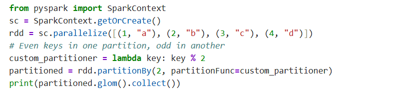
Custom partitioners
Targeted Distribution: You can control exactly where your data lives by defining a custom function that maps each key to a specific partition index (e.g., all 'A' keys to partition 0).
Performance: This is critical for optimizing joins and aggregations by ensuring related data (like all logs for one User ID) stays on the same machine, minimizing network shuffling.
Implementation: In PySpark, simply pass your custom function and the number of partitions to the partitionBy() method on a key-value Pair RDD.
Advanced transformations (mapPartitions, cogroup)
Batch Processing (mapPartitions): Unlike map which processes one row at a time, mapPartitions gives your function an iterator for the entire partition, allowing you to do heavy initialization (like opening a database connection) just once per partition.

Efficient Grouping (cogroup): This transformation groups data from two different RDDs that share the same key, returning an iterator of values for each RDD, which is the foundational building block for joins.

Yielding Results: When using mapPartitions, your function must return an iterator (using yield in Python) so Spark can pull records one by one without loading the whole partition into memory
Pair RDD operations
Key-Value Specific: Pair RDDs are simply RDDs containing tuples (key, value), which unlock special operations like reduceByKey, groupByKey, and join.
Aggregation: reduceByKey is far superior to groupByKey because it combines values locally on each mapper before sending data across the network, reducing traffic.
Joins: You can perform standard database-style joins (inner, leftOuter, rightOuter) directly on RDDs using keys to match records from two datasets.

RDD lineage and DAG
Logical Execution Plan: RDD Lineage is a graph (DAG) that records the series of transformations used to build an RDD, allowing Spark to reconstruct lost data by re-running those steps.
Fault Tolerance: If a node fails and a partition is lost, Spark looks at the lineage graph to see exactly which operations (like map -> filter) are needed to recompute just that missing slice.
Debugging: You can view this graph using toDebugString(), which prints the logical plan showing dependencies and shuffle boundaries.

Checkpoint and recovery
Truncating Lineage: checkpoint() saves the RDD data to a reliable storage (like HDFS) and cuts the lineage graph, preventing stack overflow errors in very long iterative algorithms.
Difference from Cache: Unlike cache() (which keeps lineage for recomputation), checkpoint() forgets the lineage entirely because the data is now safely stored on disk.
Directory Setup: You must set a checkpoint directory using sc.setCheckpointDir() before invoking the method.

Summary
Distributed Architecture: PySpark operates on a master-slave architecture where a Driver program translates user code into jobs, which are then executed in parallel by worker nodes (Executors) managed by a Cluster Manager.
Lazy Execution Model: The engine uses lazy evaluation, meaning transformations (like filtering or mapping) are not executed immediately but instead build a logical plan (DAG) that is only processed when an "action" (like count or write) is triggered.
Core Data Structures: Data is primarily handled using DataFrames, which are optimized distributed collections with schemas, while RDDs provide low-level control, and Datasets offer type safety for complex applications.
Unified Entry Point: The SparkSession serves as the single entry point for programming, replacing older context managers, while the underlying SparkContext connects the application to the cluster environment.
Data Ingestion & Output: PySpark supports reading and writing diverse data formats such as CSV, JSON, and Parquet (the recommended columnar format), as well as direct interactions with SQL databases via JDBC.
Transformation Capabilities: It provides a rich API for data manipulation, including standard SQL-like operations (select, filter, join), complex aggregations, and window functions for row-relative calculations like ranking or running totals.
Custom Logic Extension: When built-in functions differ from specific business needs, developers can register User Defined Functions (UDFs) to apply custom Python logic directly to DataFrame columns, though this incurs some serialization overhead.
Internal Optimization: The Catalyst Optimizer automatically refines logical plans (e.g., through predicate pushdown), while the Tungsten engine optimizes physical execution using CPU-efficient bytecode generation.
Performance Tuning: Efficiency is critical and managed through strategies like caching frequently used data in memory, broadcasting small tables during joins to minimize network traffic, and optimizing partition sizes.
Production Management: Reliable deployment involves careful memory configuration (balancing Driver vs. Executor RAM), handling data skew to prevent bottlenecks, and utilizing the Spark UI for monitoring and debugging jobs.
Resources
| Category | Resource | Link |
|---|---|---|
| Web Tutorials | Spark By Examples (Highly Recommended) | sparkbyexamples.com/pyspark-tutorial/ |
| Real Python: PySpark Guide | realpython.com/pyspark-intro/ | |
| GeeksforGeeks PySpark | www.geeksforgeeks.org/pyspark-tutorial/ | |
| Official Documentation | PySpark API Reference | spark.apache.org |
| Spark SQL, DataFrames and Datasets Guide | spark.apache.org | |
| Video Courses | Udemy: PySpark for Beginners | www.udemy.com/topic/pyspark/ |
| Coursera: Distributed Computing with Spark SQL | www.coursera.org/learn/spark-sql | |
| Databricks Academy (Free & Paid) | www.databricks.com/learn/training/home | |
| Books | Learning Spark, 2nd Edition (O'Reilly) | Focus: DataFrames, SQL, and MLlib |
| Spark: The Definitive Guide (O'Reilly) | Focus: Architecture, optimization, and advanced configurations | |
| Interactive Practice | Databricks Community Edition | community.cloud.databricks.com/ |
| StrataScratch | www.stratascratch.com/ |