SQL Learning Guide
Table of Contents
| Basic SQL | Intermediate SQL | Advanced SQL |
|---|---|---|
| 1. Database Fundamentals | 1. Advanced Joins | 1. Advanced Window Functions |
| 2. SQL Syntax & Basic Queries | 2. Subqueries | 2. Common Table Expressions (CTEs) |
| 3. Basic Operators | 3. Set Operations | 3. Advanced Subqueries |
| 4. Aggregate Functions | 4. String Functions | 4. Pivoting and Unpivoting |
| 5. Basic Joins | 5. Date and Time Functions | 5. Query Optimization |
| 6. Window Functions | 6. Views and Materialized Views | |
| 7. CASE Statements | 7. Stored Procedures and Functions | |
| 8. Data Definition Language (DDL) | ||
| 9. Indexes |
Basic SQL
1. Database Fundamentals
1.1 What is SQL?
SQL (Structured Query Language) is the standard programming language used to communicate with Relational Database Management Systems (RDBMS).
Think of a database like a giant digital filing cabinet. If the database is the cabinet, SQL is the set of instructions you use to open drawers, add new folders, find specific documents, or shred the ones you don't need anymore. It is declarative, meaning you tell the system what you want (e.g., "Give me all users from New York") rather than how to technically go get it.
1.2 Basic Database Concepts
Table, Row, and Column
A Table is a collection of related data held in a structured format within a database. It is very similar to an individual sheet in an Excel workbook.
Column (Field): The vertical part of the table. It represents a specific attribute or "category" of data (e.g., EmailAddress).
Row (Record): The horizontal part of the table. It represents a single, complete entry or "object" (e.g., one specific customer's entire set of info).
1.3 Primary Key vs. Foreign Key
This is the most critical concept for maintaining Data Integrity.
Primary Key (PK)
The Primary Key is a unique identifier for a record.
Rule: Every table should have one.
Rule: It must be unique (no two rows can have the same PK) and it cannot be NULL.
Example: Your Social Security Number or a unique User_ID.
Foreign Key (FK)
A Foreign Key is a column in one table that points to the Primary Key in another table. It acts as a "link" between the two.
Purpose: It ensures that you can't have an "Order" for a "Customer" that doesn't actually exist in the Customers table.
1.4 Data Types
When you create a column, you must tell the database what kind of data it will hold. This optimizes storage and prevents errors (like trying to multiply a "Date" by a "Word").
| Data Type | Description | Example |
|---|---|---|
| INT | Whole numbers only. No decimals. | 30 (Age), 500 (Stock) |
| VARCHAR | Variable Character. Used for text/strings. | 'John Doe', 'password123' |
| DATE | Stores YYYY-MM-DD. | '2024-05-20' |
| BOOLEAN | True or False (often stored as 1 or 0). | 1 (Active), 0 (Deleted) |
| DECIMAL | Exact numbers with decimals. Great for money. | 19.99 (Price) |
2. SQL Syntax & Basic Queries
2.1 The SELECT Statement
The SELECT statement is the bread and butter of SQL. It is used to fetch data from a database. Think of it as a filter that pulls specific information out of your tables.
SELECT * (The Wildcard)
The asterisk () is a wildcard character that means "all." When you use SELECT , you are telling the database to return every single column for every row in that table.
When to use it: During development or when you genuinely need to see the entire record.
The Downside: In large professional projects, using * is often discouraged because it can slow down the system by pulling unnecessary data (like pulling a user's entire bio when you only needed their username).
Selecting Specific Columns
To be more efficient, you list only the columns you actually need, separated by commas. This makes your queries faster and your results cleaner.
Now that you know how to pull data, the next step is learning how to be picky. In real projects, you rarely want all the data; you want specific slices--like "customers who haven't paid" or "products out of stock."
2.2 Filtering Data
The WHERE Clause
The WHERE clause is used to filter records. It ensures that only the rows that fulfill a specific condition are returned.
2.3 Sorting & Limiting
ORDER BY
The ORDER BY clause is used to sort the result set in either ascending or descending order. By default, SQL sorts data in ascending order.
Sorting by Text: Alphabetical (A to Z).
Sorting by Numbers: Smallest to largest.
Sorting by Dates: Earliest to latest.
2.4 LIMIT / OFFSET
In professional projects, tables can have millions of rows. You rarely want to pull all of them at once.
LIMIT
LIMIT specifies the maximum number of rows you want the query to return. It is incredibly useful for performance and for features like "Top 5" lists.
-- Get the 3 most expensive products
SELECT ProductName, Price
FROM Products
ORDER BY Price DESC
LIMIT 3;
OFFSET
OFFSET tells the database to skip a specific number of rows before it starts returning data.
Real-World Use Case: Pagination
When you click "Page 2" on a website search result, the code behind the scenes is using LIMIT and OFFSET.
-- Skip the first 10 results and show the next 10 (Page 2)
SELECT * FROM Products
ORDER BY ProductID
LIMIT 10 OFFSET 10;
3. Basic Operators
3.1 Comparison Operators
These are used to compare a column's value against a specific value.
| Operator | Description | Example |
|---|---|---|
| = | Equal to | WHERE status = 'active' |
| != or <> | Not equal to | WHERE role != 'admin' |
| < / > | Less than / Greater than | WHERE price < 100 |
| <= / >= | Less than or equal / Greater than or equal | WHERE age >= 21 |
3. 2 Logical Operators
Logical operators allow you to combine multiple conditions to create complex filters.
AND: Displays a record if all the conditions separated by AND are TRUE.
OR: Displays a record if any of the conditions separated by OR are TRUE.
NOT: Displays a record if the condition(s) is NOT TRUE.
-- Example: Active users who are either from New York or London
SELECT * FROM users
WHERE status = 'active'
AND (city = 'New York' OR city = 'London');
3.3 Range, List, and Pattern Operators
These operators make your queries more readable and powerful than using basic comparisons.
1. IN Operator
Allows you to specify multiple values in a WHERE clause. It is shorthand for multiple OR conditions.
2. BETWEEN Operator
Selects values within a given range (the values are inclusive: it includes the start and end).
3. LIKE Operator
Used for pattern matching with strings. It uses two "wildcards":
%: Represents zero, one, or multiple characters.
_: Represents a single character.
-- Find names starting with 'A'
SELECT * FROM employees WHERE name LIKE 'A%';

-- Find names with 'o' as the second letter
SELECT * FROM employees WHERE name LIKE '_o%';
3. 4 Null Value Operators
In SQL, NULL represents "missing" or "unknown" data. Because NULL is not a value, you cannot use = or != with it.
IS NULL: Tests for empty values.
IS NOT NULL: Tests for values that are not empty.
-- Find customers who haven't provided an email address
SELECT * FROM customers
WHERE email IS NULL;
4. Aggregate Functions
Aggregate functions perform a calculation on a set of values and return a single value. They are almost always used in conjunction with the GROUP BY clause.
1 Core Functions
| Function | Description | Example |
|---|---|---|
| COUNT() | Returns the number of rows. | COUNT(*) counts all; COUNT(col) ignores NULLs. |
| SUM() | Calculates the total of a numeric column. | SUM(salary) |
| AVG() | Calculates the arithmetic mean. | AVG(price) |
| MIN() | Finds the smallest value. | MIN(order_date) (Earliest) |
| MAX() | Finds the largest value. | MAX(age) (Oldest) |
4. 2 The GROUP BY Clause
The GROUP BY statement is used to arrange identical data into groups. It follows the WHERE clause but precedes ORDER BY.
How it Works
When you use an aggregate function, the database needs to know the "scope" of that calculation. Without GROUP BY, the scope is the entire table. With GROUP BY, the scope is each unique value in the specified column.
Example: Total Sales per Department
The "Selection Rule": If you SELECT a column that isn't inside an aggregate function (like SUM or COUNT), it must appear in the GROUP BY clause. If you forget this, the database won't know which specific row's value to display for that group.
4.3 The HAVING Clause
The HAVING clause was specifically created because the WHERE keyword cannot be used with aggregate functions.
WHERE vs. HAVING
WHERE: Filters rows before they are grouped. (e.g., "Only look at sales from 2024").
HAVING: Filters groups after they have been aggregated. (e.g., "Only show departments that made more than $10,000").
Example: Complex Filtering
SELECT city, COUNT(customer_id) AS total_customers
FROM customers
WHERE country = 'USA'            -- 1. Filter rows
GROUP BY city                    -- 2. Group rows
HAVING COUNT(customer_id) > 5;   -- 3. Filter groups
Summary Checklist for Aggregation
Use COUNT(DISTINCT column) if you want to count unique items only (like unique customers).
Use NULL handling: Remember that SUM, AVG, MIN, and MAX ignore NULL values.
Logical Flow: Always think of the order: Filter (WHERE) -> Group (GROUP BY) -> Filter Groups (HAVING).
5. Basic Joins
A JOIN clause is used to combine rows from two or more tables, based on a related column between them. Usually, this relationship is built between a Primary Key in one table and a Foreign Key in another.
5. 1 INNER JOIN
The INNER JOIN is the "strict" join. It only returns rows where there is a match in both tables. If a record in the first table doesn't have a corresponding match in the second, it is excluded from the results.
SELECT orders.order_id, customers.customer_name
FROM orders
INNER JOIN customers
ON orders.customer_id = customers.customer_id;
Result: A list of orders along with the names of the customers who placed them. If a customer hasn't ordered anything, they won't appear here.
Of course, sometimes you want to see the "lonely" data too--like the customers who haven't spent a dime yet--which brings us to Outer Joins.
5. 2 LEFT JOIN (Left Outer Join)
The LEFT JOIN returns all records from the left table (the one listed first), and the matched records from the right table. If there is no match, the result from the right side will be NULL.
SELECT customers.customer_name, orders.order_id
FROM customers
LEFT JOIN orders
ON customers.customer_id = orders.customer_id;
Result: A full list of every customer. If they have orders, you see the order_id. If they don't, the order_id column will simply say NULL.
5.3 RIGHT JOIN (Right Outer Join)
The RIGHT JOIN is simply the mirror image of the Left Join. It returns all records from the right table and the matched records from the left.
Reality Check: In the professional world, RIGHT JOIN is rarely used. Most developers find it easier to read a query from left-to-right, so they simply flip the table order and use a LEFT JOIN instead.
Now that we know the types of joins, we need to talk about the "glue" that holds them together: the join condition.
5.4 Understanding Join Conditions (ON Clause)
The ON clause is where you define the logic for the connection. While 90% of joins use the equals operator (=), you are essentially telling the database: "Link these two rows if the data in Column A matches the data in Column B."
Important Distinctions:
ON vs. WHERE: Use ON for the logic that links the tables together. Use WHERE to filter the results after they've been linked.
Table Aliases: When joining, table names get long. Use aliases to save your fingers.
Instead of: orders.customer_id
Use: o.customer_id (by defining FROM orders AS o)
Pro Tip: Always prefix your column names with the table name (or alias) when joining. If both tables have a column named id or created_at and you just type SELECT id, the database will get "ambiguous column" anxiety and throw an error.
Imagine a scenario where we want a report of all customers, their orders, and the products they bought, but only for high-value items.
The "All-in-One" Basic Join Query
SELECT
c.customer_name,
c.city,
o.order_date,
p.product_name,
p.price
FROM customers AS c                             -- Left Table
LEFT JOIN orders AS o                           -- 1. LEFT JOIN (Includes customers with no orders)
ON c.customer_id = o.customer_id            -- Join Condition
INNER JOIN products AS p                        -- 2. INNER JOIN (Only matches orders that have valid products)
ON o.product_id = p.product_id              -- Join Condition
WHERE p.price > 100                             -- 3. Filtering
ORDER BY o.order_date DESC;                     -- 4. Sorting
Breaking Down the Concepts
Table Aliasing (AS c, AS o): Notice how we used shortcuts for table names. This prevents the query from becoming a massive wall of repetitive text and makes it easier to read.
The ON Clause: This is the bridge. We are explicitly telling SQL that the customer_id in the customers table is the exact same piece of data as the customer_id in the orders table.
Mixing Join Types: * The LEFT JOIN ensures we see every customer (even the window shoppers who haven't bought anything).
The INNER JOIN ensures that if an order exists, it must have a matching product to be included in this specific list.
Logical Execution: SQL first builds the massive combined table using the JOIN logic, then trims it down using your WHERE clause, and finally organizes it with ORDER BY.
Intermediate SQL
1. Advanced Joins
1.1 FULL OUTER JOIN
A FULL OUTER JOIN returns all records when there is a match in either the left or the right table. It’s essentially a combination of a LEFT JOIN and a RIGHT JOIN.
The Result: You get a complete view of both tables. Where there is no match, you will see NULL values on either side.
Use Case: Synchronizing two different databases (e.g., finding which customers are in your CRM but not in your Mailing List, and vice-versa).
While Full Joins show you everything that exists, sometimes you need to generate data that doesn't exist yet--enter the Cross Join.
1.2 CROSS JOIN (The Cartesian Product)
A CROSS JOIN produces a result set which is the number of rows in the first table multiplied by the number of rows in the second table.
The Catch: You do not use an ON clause. Every row from Table A is paired with every row from Table B.
Use Case: If you have 3 Shirt Colors and 3 Shirt Sizes, a CROSS JOIN will generate all 9 possible combinations for your inventory.
1.3 Self Joins
A Self Join is a regular join, but the table is joined with itself. To do this, you must use table aliases to give the table two different "nicknames."
Use Case: Hierarchy data. For example, an Employees table where one column (manager_id) refers back to the employee_id in the same table.
SELECT
e.name AS Employee,
m.name AS Manager
FROM employees AS e
INNER JOIN employees AS m
ON e.manager_id = m.employee_id;
1.4 Multiple Table Joins
In real-world applications, data is often spread across four or five tables. You simply chain the JOIN commands one after the other.
SELECT c.name, o.order_date, p.product_name, s.supplier_name
FROM customers c
JOIN orders o ON c.id = o.customer_id
JOIN products p ON o.product_id = p.id
JOIN suppliers s ON p.supplier_id = s.id;
Connecting five tables is great, but doing it poorly can bring a database to its knees. Let’s talk about keeping things fast.
1.5 Join Optimization
As your data grows, joins can become slow. Here is how to keep them snappy:
Index Your Keys: Ensure that any column used in an ON clause (Primary and Foreign Keys) has an Index. This is the single biggest performance booster.
Filter Early: Use WHERE clauses to reduce the number of rows before the join happens if possible.
Join Order: Start with the smallest table (after filtering) to reduce the "work" the database has to do in subsequent joins.
Avoid SELECT *: Every extra column you pull through a join consumes memory and bandwidth.
2. Subqueries
2.1 Subqueries in the WHERE Clause
This is the most common use case. You use the inner query to find a value (or a list of values) that the outer query then uses to filter its results.
Example: Find all products that are priced higher than the average price.
The Logic: The database first calculates the AVG(price), then uses that single number to filter the outer list.
Of course, filtering isn't the only way to use a nested query; sometimes you want that data to appear right next to your main columns.
2.2 Subqueries in the SELECT Clause
You can use a subquery to create a calculated column for every row in your result set.
Example: Show each employee's name and the total number of orders they have handled.
SELECT
name,
(SELECT COUNT(*) FROM orders WHERE orders.employee_id = employees.id) AS order_count
FROM employees;
2.3 Subqueries in the FROM Clause (Derived Tables)
When you put a subquery in the FROM clause, you are essentially creating a temporary table that exists only for that query. You must give these subqueries an alias.
Example: Find the maximum average salary across different departments.
SELECT MAX(avg_sal)
FROM (
SELECT department, AVG(salary) AS avg_sal
FROM employees
GROUP BY department
) AS dept_averages;
While the subqueries above run once and finish, some subqueries are a bit more "talkative" with the outer query.
2.4 Correlated Subqueries
A correlated subquery is a subquery that uses values from the outer query. It executes once for every row processed by the outer query, making it powerful but potentially slower.
Example: Find employees who earn more than the average salary of their specific department.
SELECT name, salary, department
FROM employees AS e1
WHERE salary > (
    SELECT AVG(salary)
    FROM employees AS e2
    WHERE e2.department = e1.department
);
The Logic: For every employee in e1, the subquery re-calculates the average for their specific department.
Summary Checklist for Subqueries
| Placement | Purpose | Note |
|---|---|---|
| WHERE | To filter results based on dynamic values. | Often used with IN, ANY, or ALL. |
| SELECT | To add a summary or lookup value to each row. | Can be slow if the table is very large. |
| FROM | To treat a query result like a real table. | Must always have an AS alias. |
| Correlated | To compare a row against its own "peer group." | Referencing the outer table inside the inner query. |
Pro Tip: If you find yourself nesting subqueries more than two levels deep, the code becomes very hard to read. In those cases, you should switch to CTEs (Common Table Expressions) using the WITH keyword, which we'll cover in the next section!
3. Set Operations
To use any set operation, you must follow two strict rules:
Both queries must have the same number of columns.
The columns must have compatible data types in the same order.
3.1 UNION and UNION ALL
UNION combines the result sets of two SELECT statements.
UNION: Merges the lists and removes duplicates. It’s like a "Unique" filter for your combined data.
UNION ALL: Merges the lists and keeps everything, including duplicates.
-- Get a list of all unique cities where we have either customers or suppliers
SELECT city FROM customers
UNION
SELECT city FROM suppliers;
While UNION combines everything, sometimes you only want to see the overlap--where two groups actually meet.
3.2 INTERSECT
The INTERSECT operator returns only the rows that are present in both query results.
Use Case: Finding "Common Ground." For example, finding customers who are also registered as employees.
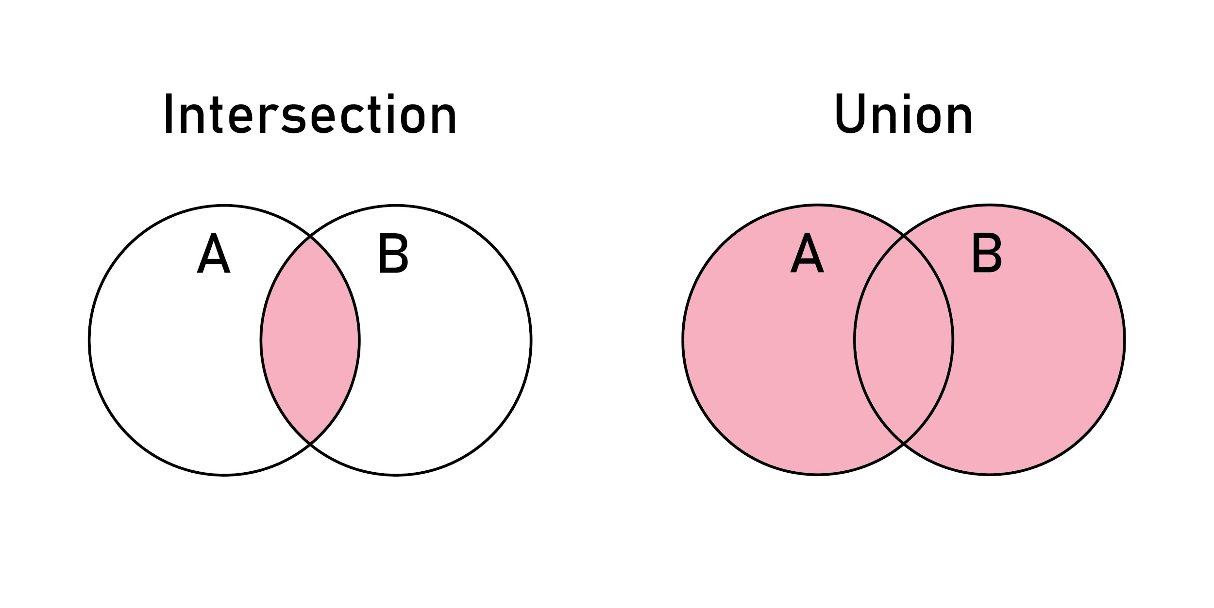
-- Find cities that have BOTH a warehouse AND a retail store
SELECT city FROM warehouses
INTERSECT
SELECT city FROM retail_stores;
3.3 EXCEPT / MINUS
This operator returns the rows from the first query that are not present in the second query.
Note: Oracle and some others use MINUS, while SQL Server and PostgreSQL use EXCEPT.
Use Case: Finding "The Exceptions." For example, finding products that have been created but have never been ordered.
-- Find products that have NEVER been sold
SELECT product_id FROM products
EXCEPT
SELECT product_id FROM orders;
Summary Checklist for Set Operations
| Operation | Logic | Duplicate Handling |
|---|---|---|
| UNION | Combine results | Removes duplicates (Slower) |
| UNION ALL | Combine results | Keeps duplicates (Faster) |
| INTERSECT | Common to both | Only keeps matches |
| EXCEPT | In A, but not in B | Removes B's data from A |
4. String Functions
4.1 CONCAT, SUBSTRING, LENGTH
These functions help you build or dismantle strings to get exactly the text you need.
CONCAT(str1, str2, ...): Joins two or more strings together.
SUBSTRING(str, start, length): Extracts a specific portion of a string.
LENGTH(str) (or LEN in SQL Server): Returns the number of characters in a string.
Now that you've reshaped the text, you often need to standardize it--because to a database, 'Admin' and 'admin' aren't always the same thing.
4.2 UPPER, LOWER, TRIM
These are essential for data cleaning and ensuring consistent formatting.
UPPER(str) / LOWER(str): Converts text to all caps or all lowercase. Great for case-insensitive searches.
TRIM(str): Removes leading and trailing spaces.
Pro Tip: Use LTRIM or RTRIM if you only want to clean one specific side.
Sometimes you don't just want to change the case; you need to find a needle in a haystack or swap one word for another.
4.3 REPLACE, CHARINDEX / POSITION
These functions allow you to search within strings and modify specific parts of them.
REPLACE(str, old, new): Finds all occurrences of a sub-string and replaces them with something else.
CHARINDEX(find, str) (SQL Server) or POSITION(find IN str) (PostgreSQL): Returns the starting position of a specific character or word.
Example: Finding where the '@' symbol is in an email to extract the domain.
Summary Checklist for Strings
| Goal | Function to Use |
|---|---|
| Join Text | CONCAT() |
| Change Case | UPPER() / LOWER() |
| Clean Spaces | TRIM() |
| Get Part of Text | SUBSTRING() |
| Find Location | CHARINDEX() / POSITION() |
Pro Tip: When using SUBSTRING and CHARINDEX together, you can perform powerful "dynamic" cleaning. For example, to get everything after the '@' in an email:
5. Date and Time Functions
5.1 DATE and DATETIME Operations
Databases store time in specific formats, most commonly:
DATE: YYYY-MM-DD (e.g., 2026-02-12)
DATETIME / TIMESTAMP: YYYY-MM-DD HH:MM:SS
You can compare dates just like numbers. WHERE order_date > '2025-01-01' works perfectly fine because SQL understands the chronological order of these strings.
Comparing dates is easy, but shifting them forward or backward--like calculating a 30-day expiration--requires a bit more "math."
5.2 DATE_ADD, DATE_SUB, and DATEDIFF
These functions allow you to perform "date arithmetic."
DATE_ADD(date, INTERVAL value unit): Adds time to a date.
DATE_SUB(date, INTERVAL value unit): Subtracts time from a date.
DATEDIFF(date1, date2): Returns the number of days between two dates.
5.3 EXTRACT and DATE_PART
Sometimes you don't need the whole date; you just need to know which month a sale happened in or what time of day your server is busiest.
EXTRACT(unit FROM date): Pulls a specific part (YEAR, MONTH, DAY, HOUR) out of the date.
DATE_PART: The PostgreSQL equivalent of extract.
-- Finding which month has the most signups
SELECT EXTRACT(MONTH FROM signup_date) AS signup_month, COUNT(*)
FROM users
GROUP BY signup_month;
Pulling parts of a date is great for logic, but when it's time to show those results to a human, you'll want it to look a bit prettier than 2026-02-12.
5.4 Date Formatting
Formatting functions turn raw date data into readable strings like "Thursday, February 12th."
MySQL: DATE_FORMAT(date, '%W, %M %e')
SQL Server: FORMAT(date, 'D')
PostgreSQL: TO_CHAR(date, 'Day, Month DD')
-- Formatting a date for a front-end report
SELECT DATE_FORMAT(created_at, '%M %Y') AS formatted_date FROM blog_posts;
-- Result: "February 2026"
Summary Checklist for Dates
| Goal | Function (Commonly) |
|---|---|
| Get Today's Date | CURRENT_DATE or NOW() |
| Find Difference | DATEDIFF() |
| Add/Remove Time | DATE_ADD() / DATE_SUB() |
| Get Just the Year | EXTRACT(YEAR FROM date) |
| Change Appearance | DATE_FORMAT() / TO_CHAR() |
Pro Tip: Always store your dates in UTC (Coordinated Universal Time). It is much easier to convert a UTC timestamp to a user's local timezone for display than it is to fix a database where half the entries are in EST and the other half are in PST.
6. Window Functions
6.1 The OVER Clause and PARTITION BY
The OVER clause defines the "window" of rows the function should look at.
OVER(): Looks at the entire result set.
PARTITION BY: Breaks the data into groups (like GROUP BY), but keeps the individual rows visible.
Once you've defined the window, you usually want to give each row a specific place in line.
6.2 ROW_NUMBER(), RANK(), and DENSE_RANK()
These are "Ranking Functions" used to assign a number to each row based on a specific order.
ROW_NUMBER(): Assigns a unique, sequential number to each row (1, 2, 3, 4).
RANK(): Assigns the same number to tied values, but skips the next number (1, 2, 2, 4).
DENSE_RANK(): Assigns the same number to ties, but does not skip numbers (1, 2, 2, 3).
SELECT
name,
salary,
department,
RANK() OVER(PARTITION BY department ORDER BY salary DESC) AS salary_rank
FROM employees;
Ranking is great for leaderboards, but sometimes you need to see how a single row compares to the group's total without losing that row's identity.
6.3 Aggregation in Window Functions
You can use standard aggregates like SUM(), AVG(), and COUNT() as window functions. This is incredibly useful for creating running totals or comparing a value to a department average.
Example: Creating a Running Total
Summary Comparison: GROUP BY vs. Window Functions
| Feature | GROUP BY | Window Function (OVER) |
|---|---|---|
| Row Count | Reduces rows to summaries. | Keeps all original rows. |
| Usage | High-level reporting. | Detailed analysis & row-level comparisons. |
| Syntax | GROUP BY column | AGG() OVER(PARTITION BY column) |
Pro Tip: Window functions are processed after the WHERE clause. This means you can't filter by a window function result (like salary_rank) in the same query. You'll need to wrap it in a CTE or Subquery to filter based on the rank!
Example 1: Finding the "Top N" Records per Group
A common task is finding the top performers in every category (e.g., the top 2 most expensive products in every category). We'll use a CTE combined with DENSE_RANK() to make this readable.
WITH RankedProducts AS (
    SELECT
        product_name,
        category,
        price,
        DENSE_RANK() OVER(PARTITION BY category ORDER BY price DESC) AS price_rank
    FROM products
)
-- Now we can filter by the rank we created
SELECT * FROM RankedProducts
WHERE price_rank <= 2;
Ranking gives you a snapshot of who is winning, but calculating growth requires looking at the data as a continuous stream.
Example 2: Monthly Revenue with a Running Total
This query uses a Window Function to calculate a Running Total (Cumulative Sum) of revenue over time. This is the foundation for creating those growth charts you see in business dashboards.
SELECT
    order_date,
    SUM(sale_amount) AS daily_revenue,
    SUM(SUM(sale_amount)) OVER (ORDER BY order_date) AS cumulative_revenue
FROM orders
GROUP BY order_date
ORDER BY order_date;
How this works:
The inner SUM(sale_amount) calculates the total for each day.
The outer SUM(...) OVER(...) takes those daily totals and adds them to the previous days' totals as it moves down the list.
Summary of Advanced Analysis
| If you want to... | Use this Tool |
|---|---|
| Assign a unique ID to duplicates | ROW_NUMBER() |
| Handle ties in a leaderboard | RANK() or DENSE_RANK() |
| Calculate a % of a total | SUM(x) / SUM(x) OVER() |
| Compare row vs. group average | AVG(x) OVER(PARTITION BY category) |
Pro Tip: When using OVER(ORDER BY ...), SQL defaults the "window frame" to include all rows from the start of the partition up to the current row. This is why it creates a running total automatically. If you leave out the ORDER BY, it will just give you the grand total for every row!
7. CASE Statements
CASE statements are the "If-Then-Else" logic of the SQL world. They allow you to add conditional logic directly into your queries, making it possible to categorize data or handle exceptions on the fly.
7.1 Simple CASE Expressions
A simple CASE compares one expression to a set of simple values to determine the result.
SELECT product_name,
CASE category_id
WHEN 1 THEN 'Electronics'
WHEN 2 THEN 'Clothing'
ELSE 'Other'
END AS category_name
FROM products;
Simple CASE is great for direct matches, but when your logic gets more complex--like checking price ranges--you'll need the Searched version.
7.2 Searched CASE Expressions
The Searched CASE is more powerful because it allows you to use comparison operators (>, <, LIKE, IN) in your conditions.
Example: Tiering Customers by Spend
SELECT customer_name, total_spent,
    CASE
        WHEN total_spent > 10000 THEN 'Platinum'
        WHEN total_spent BETWEEN 5000 AND 10000 THEN 'Gold'
        WHEN total_spent > 0 THEN 'Silver'
        ELSE 'Lead'
    END AS customer_tier
FROM customers;
While CASE handles logic, sometimes you just need to handle "missingness." This is where the specialized cousins of the CASE statement come in.
7.3 COALESCE and NULLIF
These are shorthand functions for specific types of conditional logic.
COALESCE(val1, val2, ...): Returns the first non-null value in the list. It’s perfect for providing default values.
NULLIF(val1, val2): Returns NULL if the two values are equal. This is most commonly used to prevent Division by Zero errors.
Summary Checklist for Logic
| Function | Best Use Case |
|---|---|
| Simple CASE | Mapping IDs to labels. |
| Searched CASE | Ranges (Age, Price, Dates). |
| COALESCE | Filling in "Missing" (NULL) values. |
| NULLIF | Safety checks for math operations. |
Pro Tip: You can use CASE statements inside aggregate functions! This is called Conditional Aggregation. For example: SUM(CASE WHEN status = 'shipped' THEN 1 ELSE 0 END) gives you a count of shipped items without needing a separate WHERE clause.
Example 1: Creating a "Pivot" Report (Conditional Aggregation)
Instead of having rows for every status, you can use CASE inside a SUM function to create columns for each status. This is a classic "Executive Dashboard" pattern.
SELECT
EXTRACT(MONTH FROM order_date) AS month,
SUM(CASE WHEN status = 'Completed' THEN 1 ELSE 0 END) AS successful_orders,
SUM(CASE WHEN status = 'Cancelled' THEN 1 ELSE 0 END) AS lost_orders,
SUM(CASE WHEN status = 'Refunded' THEN 1 ELSE 0 END) AS refund_count
FROM orders
GROUP BY month;
Transforming rows into columns is a great way to summarize data, but sometimes you need the logic to handle the "unknowns" in your contact list.
Example 2: Data Cleanup with COALESCE and CASE
Imagine a table where contact info is scattered across three different columns (Mobile, Work, Home). You want to find the best way to reach them in a specific order of priority.
SELECT
    name,
    COALESCE(mobile_phone, work_phone, home_phone, 'No Contact Found') AS primary_contact,
    CASE
        WHEN mobile_phone IS NOT NULL THEN 'Mobile'
        WHEN work_phone IS NOT NULL THEN 'Work'
        WHEN home_phone IS NOT NULL THEN 'Home'
        ELSE 'N/A'
    END AS contact_source
FROM users;
8. Data Definition Language (DDL)
8.1 CREATE TABLE
This is the command used to build a new table from scratch. You must define the column names, their data types, and any initial constraints.
CREATE TABLE employees (
employee_id INT PRIMARY KEY,         -- Unique ID for every row
first_name VARCHAR(50) NOT NULL,     -- Cannot be empty
email VARCHAR(100) UNIQUE,           -- No two people can have the same email
salary DECIMAL(10, 2) DEFAULT 0.00,  -- If no salary is provided, it defaults to 0
hire_date DATE DEFAULT CURRENT_DATE  -- Defaults to today's date
);
Of course, business needs evolve. You might start with five columns and realize six months later that you forgot to track "Department."
8.2 ALTER TABLE
Use ALTER to modify the structure of an existing table without losing your data.
ADD: ALTER TABLE employees ADD department VARCHAR(30);
MODIFY: ALTER TABLE employees MODIFY salary DECIMAL(12, 2);
DROP: ALTER TABLE employees DROP COLUMN hire_date;
8.3 DROP TABLE
This is the most "dangerous" command in SQL. It deletes the table structure and all the data inside it permanently.
Building a table is easy, but keeping it "clean" requires rules. These rules are called Constraints.
8.4 SQL Constraints
Constraints are the "guardrails" that prevent bad data from entering your database.
| Constraint | Purpose | Example |
|---|---|---|
| PRIMARY KEY | Uniquely identifies each row. Cannot be NULL. | id INT PRIMARY KEY |
| UNIQUE | Ensures all values in a column are different. | passport_no VARCHAR(20) UNIQUE |
| CHECK | Ensures values satisfy a specific condition. | CHECK (age >= 18) |
| DEFAULT | Sets a value if none is provided. | status VARCHAR(10) DEFAULT 'Active' |
| NOT NULL | Ensures a column cannot have a NULL value. | username VARCHAR(50) NOT NULL |
Putting it All Together: A Robust Table Design
CREATE TABLE product_inventory (
sku_id INT PRIMARY KEY,
product_name VARCHAR(255) NOT NULL,
stock_level INT DEFAULT 0,
price DECIMAL(10, 2),
-- Constraint: Price must be positive
CONSTRAINT chk_positive_price CHECK (price > 0),
-- Constraint: Names must be unique to prevent double entry
CONSTRAINT uq_product_name UNIQUE (product_name));
9. Indexes
9.1 Basic Index Concepts
An index is a separate data structure (usually a B-Tree) that stores a sorted version of a column’s data along with a pointer to the original row.
Search Speed: Drastically reduces the time to find rows using WHERE or JOIN.
The Trade-off: Every time you INSERT, UPDATE, or DELETE, the database also has to update the index. This makes writes slightly slower to make reads significantly faster.
While primary keys get indexes automatically, your search patterns usually dictate where you should manually build more.
9.2 Creating Indexes
There are two main types of indexes you will create:
Standard Index: Used for columns you frequently search by (like last_name).
Unique Index: Not only speeds up searches but also acts as a constraint, preventing duplicate values.
It is tempting to index everything to make the whole database "fast," but that's a trap that can actually tank your performance.
9.3 When to Use Indexes
Knowing when not to use an index is just as important as knowing when to use one.
Use an Index when:
A column is frequently used in WHERE clauses.
A column is used for JOIN operations (Foreign Keys).
A column is used for ORDER BY or GROUP BY.
The table is large (thousands or millions of rows).
Avoid an Index when:
The table is very small (it's faster for the DB to just read the whole thing).
The column has very low "cardinality" (e.g., a "Gender" column where values are only M, F, or O).
The table is "write-heavy" (e.g., a log table that is updated 100 times per second).
Summary Checklist for Performance
| Feature | Primary Key | Standard Index |
|---|---|---|
| Creation | Automatic | Manual |
| Duplicates | Not Allowed | Allowed |
| Nulls | Not Allowed | Allowed |
| Limit | One per table | Many per table |
Pro Tip: Beware of Over-Indexing. If you have a table with 10 columns and 10 indexes, your INSERT statements might take twice as long as they should. Aim for "The Goldilocks Zone"--only index the columns that are actually part of your frequent query patterns.
Example 1: The "Composite" Index
Sometimes you don't just search by one column; you search by a combination. For example, a retail database searching for orders based on both store_id and status.
-- Creating a composite index on two columns
-- This query is now lightning fast because the index covers both filters
While composite indexes handle multiple columns, sometimes the data inside a single column is so large that you only need to index the beginning of it.
Example 2: The "Covering" Index
A "Covering Index" is an index that includes all the columns requested by a query. If the index has all the answers, the database doesn't even have to look at the actual table!
-- If we frequently run this specific query:
-- We create an index that "covers" both columns
Advanced SQL
1. Advanced Window Functions
1.1 LAG and LEAD
These are the most popular advanced functions. They allow you to access data from a previous row (LAG) or a subsequent row (LEAD) relative to the current row.
Use Case: Calculating "Month-over-Month" growth.
Syntax: LAG(column, offset, default_value)
SELECT
month,
revenue,
LAG(revenue, 1) OVER (ORDER BY month) AS prev_month_revenue,
revenue - LAG(revenue, 1) OVER (ORDER BY month) AS month_diff
FROM monthly_sales;
Accessing the neighbor next door is useful, but sometimes you need to pinpoint the "extreme" values within a specific partition.
1.2 FIRST_VALUE, LAST_VALUE, and NTH_VALUE
These functions allow you to grab specific values from the "window" of rows you've defined.
FIRST_VALUE(col): Grabs the value from the very first row in the window.
LAST_VALUE(col): Grabs the value from the very last row in the window.
NTH_VALUE(col, n): Grabs the value from the row at position n.
1.3 Window Frames (ROWS vs. RANGE)
This is the most misunderstood part of window functions. A "frame" tells SQL exactly which rows to include in the calculation relative to the current row.
ROWS BETWEEN 3 PRECEDING AND CURRENT ROW: Only looks at the last 3 rows plus the current one.
UNBOUNDED PRECEDING: Means "from the very beginning of the partition."
-- Calculating a 7-day moving average
SELECT
sale_date,
amount,
AVG(amount) OVER (
ORDER BY sale_date
ROWS BETWEEN 6 PRECEDING AND CURRENT ROW
) AS moving_avg_7d
FROM sales;
Once you can control the frame, you can move from simple totals to sophisticated statistical distributions.
1.4 Percentile Functions (NTILE, PERCENT_RANK)
These functions help you understand the distribution of your data.
NTILE(n): Divide your data into n equal buckets. NTILE(4) creates quartiles.
PERCENT_RANK(): Returns the relative rank of a row as a percentage (from 0 to 1).
1.5 Example: The "Super-Analytic" Query
Let's combine these into a real-world scenario: Analyzing stock prices to find daily changes and the "Top 25%" threshold.
-- 1. Get previous day's price
-- 2. Calculate the "Running Max"
-- 3. Divide prices into 4 quartiles
Pro Tip: Be careful with LAST_VALUE. By default, the window frame is RANGE BETWEEN UNBOUNDED PRECEDING AND CURRENT ROW. This means LAST_VALUE will just return the value of the current row! To get the true last value of a partition, you must specify ROWS BETWEEN UNBOUNDED PRECEDING AND UNBOUNDED FOLLOWING.
To really master advanced window functions, you need to see how they handle trends and outliers. These are the queries that turn "raw numbers" into "business intelligence."
Example 1: Calculating "Time-To-Conversion"
A classic marketing analytics question: "How much time passed between this user's current session and their previous session?" This is perfect for LAG().
SELECT
    user_id,
    session_timestamp,
    -- Get the time of the previous session for the same user
    LAG(session_timestamp) OVER (
        PARTITION BY user_id
        ORDER BY session_timestamp
    ) AS last_session,
    -- Calculate the difference in hours
    DATEDIFF(
        session_timestamp,
        LAG(session_timestamp) OVER (PARTITION BY user_id ORDER BY session_timestamp)
    ) AS hours_since_last_visit
FROM user_sessions;
Calculating time gaps is great for behavioral analysis, but if you're looking at performance, you often want to see how the current row stacks up against the "Gold Standard" of the group.
Example 2: Comparing Every Row to the Best Performer
Let’s say you want to see every salesperson's revenue and exactly how much they are trailing behind the top performer in their specific region.
SELECT
    region,
    salesperson_name,
    revenue,
    -- Find the highest revenue in the region
    FIRST_VALUE(revenue) OVER (
        PARTITION BY region
        ORDER BY revenue DESC
    ) AS regional_best,
    -- Calculate the "Gap to Top"
    FIRST_VALUE(revenue) OVER (PARTITION BY region ORDER BY revenue DESC) - revenue AS gap_to_leader
FROM sales_performance;
Pro-Tip: The "Running Average" vs. "Moving Average" - There is a subtle but massive difference between these two in SQL:
Running Average: Use ROWS UNBOUNDED PRECEDING. This averages everything from the beginning of time until now. It gets "smoother" and slower to change as you add data.
Moving Average: Use ROWS BETWEEN 10 PRECEDING AND CURRENT ROW. This only looks at a specific window (like the last 10 days). It is much more responsive to recent trends.
2. Common Table Expressions (CTEs)
2.1 Simple CTEs
A simple CTE uses the WITH keyword to define a temporary table. This makes your main query much easier to read because the complex logic is moved to the top.
WITH HighValueOrders AS (
    SELECT customer_id, SUM(amount) AS total_spent
    FROM orders
    GROUP BY customer_id
    HAVING SUM(amount) > 1000
)
SELECT c.customer_name, hvo.total_spent
FROM customers c
JOIN HighValueOrders hvo ON c.id = hvo.customer_id;
Once you're comfortable with one CTE, you'll realize you can chain them together like a data assembly line.
2.2 Multiple CTEs
You can define multiple CTEs in a single statement by separating them with commas. Each subsequent CTE can even reference the ones defined before it!
WITH RegionalSales AS (
SELECT region, SUM(amount) AS total_revenue
FROM sales
GROUP BY region
),
TopRegions AS (
SELECT region FROM RegionalSales
WHERE total_revenue > 50000
)
SELECT * FROM orders WHERE region IN (SELECT region FROM TopRegions);
Chaining tables is powerful for linear logic, but what if your data is a loop or a tree? That's where things get recursive.
2.3 Recursive CTEs
Recursive CTEs are used to query hierarchical data, such as organizational charts (manager -> employee) or family trees. They work by repeatedly executing a query and adding the results to the previous set until a condition is met.
Structure:
Anchor Member: The starting point (e.g., the CEO).
UNION ALL: The glue connecting the levels.
Recursive Member: The query that joins the CTE back to the original table.
WITH RECURSIVE OrgChart AS (
    -- Anchor: Find the CEO
    SELECT employee_id, name, manager_id, 1 AS level
    FROM employees WHERE manager_id IS NULL

    UNION ALL

    -- Recursion: Join employees to their managers
    SELECT e.employee_id, e.name, e.manager_id, oc.level + 1
    FROM employees e
    INNER JOIN OrgChart oc ON e.manager_id = oc.employee_id
)
SELECT * FROM OrgChart ORDER BY level;
Recursive logic is heavy lifting for a database, so you need to be mindful of how you're using these tools.
2.4 CTE Optimization
Contrary to popular belief, CTEs are not always faster than subqueries.
Materialization: In some databases (like older PostgreSQL), CTEs are "materialized," meaning the DB writes the results to a temp table first. This can be slow for massive datasets.
Predicate Pushdown: Modern optimizers can often "reach into" a CTE to apply filters from the main query, but it’s not guaranteed.
Readability vs. Performance: Always prioritize CTEs for readability, but if a query is timing out, try refactoring it into a temp table or a subquery to see if the execution plan improves.
More Examples
Example 3: Finding "Above Average" Performers
Using a CTE makes it easy to compare individual rows against an aggregate value without using window functions.
WITH DeptAvg AS (
    SELECT department_id, AVG(salary) AS avg_sal
    FROM employees
    GROUP BY department_id
)
SELECT e.name, e.salary, d.avg_sal
FROM employees e
JOIN DeptAvg d ON e.department_id = d.department_id
WHERE e.salary > d.avg_sal;
Example 4: Generating a Date Series
Recursive CTEs aren't just for hierarchies; they are great for generating data on the fly, like a list of dates for a report.
WITH RECURSIVE DateRange AS (
SELECT '2026-02-01' AS report_date -- Start Date
UNION ALL
SELECT DATE_ADD(report_date, INTERVAL 1 DAY)
FROM DateRange
WHERE report_date < '2026-02-12' -- End Date
)
SELECT * FROM DateRange;
Pro Tip: In Recursive CTEs, always ensure you have a "termination condition" in the WHERE clause. If you don't, you'll create an infinite loop that will eventually crash your session (or the server!).
3. Advanced Subqueries
3.1 EXISTS and NOT EXISTS
The EXISTS operator is used to test for the existence of any record in a subquery. It is highly efficient because it stops searching the moment it finds a single match (a "short-circuit" operation).
Logic: It returns TRUE if the subquery returns one or more records.
Example: Find all customers who have placed at least one order.
SELECT customer_name
FROM customers c
WHERE EXISTS (
    SELECT 1
    FROM orders o
    WHERE o.customer_id = c.id
);
While EXISTS checks for "any" match, sometimes you need to compare a value against "every" or "some" values in a list.
3.2 ANY and ALL Operators
These operators allow you to compare a single value to a set of values returned by a subquery.
ANY: Returns true if the comparison is true for at least one value in the list (similar to OR).
ALL: Returns true if the comparison is true for every value in the list (similar to AND).
Example: Find products whose price is greater than the price of all products in the 'Basic' category.
SELECT product_name, price
FROM products
WHERE price > ALL (
    SELECT price FROM products WHERE category = 'Basic'
);
Standard subqueries are usually "self-contained," but sometimes you need the subquery to act like a FOR EACH loop that can see the columns of the outer table.
3.3 Lateral Subqueries (LATERAL / CROSS APPLY)
A LATERAL join (or CROSS APPLY in SQL Server) is essentially a subquery that can reference columns from preceding tables in the FROM clause. This allows you to perform calculations or lookups for each row individually.
Example: For each department, find the top 2 highest-paid employees.
SELECT d.dept_name, e.name, e.salary
FROM departments d
CROSS JOIN LATERAL (
    SELECT name, salary
    FROM employees
    WHERE department_id = d.id
    ORDER BY salary DESC
    LIMIT 2
) AS e;
3.4 Subquery Optimization
Advanced subqueries can be performance killers if not written carefully.
Prefer EXISTS over IN: When checking for existence in a large table, EXISTS is usually faster because it doesn't build an actual list of values in memory.
Avoid Unnecessary Correlation: Correlated subqueries (where the inner query refers to the outer) run once for every row. If you can rewrite them as a JOIN, you should.
Flattening: Modern database optimizers try to "flatten" subqueries into joins automatically, but they can't always do it for complex logic.
More Examples
Example 1: Finding "Lone Wolves" with NOT EXISTS
Find departments that currently have no employees assigned to them.
SELECT dept_name
FROM departments d
WHERE NOT EXISTS (
SELECT 1
FROM employees e
WHERE e.department_id = d.id
);
Example 2: Comparing to Group Minimums with ANY
Find any employee who earns more than at least one manager.
SELECT name, salary
FROM employees
WHERE salary > ANY (
SELECT salary FROM employees WHERE job_title = 'Manager');
Example 3: Dynamic Calculations with LATERAL
Get each product and its discount price based on a complex logic table.
SELECT p.name, p.price, d.discounted_price
FROM products p,
LATERAL (
    SELECT p.price * (1 - discount_pct) AS discounted_price
    FROM discount_rules
    WHERE p.category = category_name
    AND CURRENT_DATE BETWEEN start_date AND end_date
) AS d;
Pro Tip: When using EXISTS, the columns you select in the subquery don't matter (e.g., SELECT 1, SELECT *, SELECT 'X'). The database only cares if a row is returned, so SELECT 1 is the industry standard for readability and to show you aren't actually using the data.
4. Pivoting and Unpivoting
4.1 PIVOT Operations
Pivoting turns unique values from one column into multiple new columns. This is most commonly used to transform a list of sales transactions into a monthly or regional comparison table.
Logic: You take a categorical column (like "Month") and "rotate" its values to become headers.
The Manual Way: If your database doesn't have a native PIVOT function, you use Conditional Aggregation.
-- Standard PIVOT using CASE (Works in all SQL dialects)
SELECT
    Salesperson,
    SUM(CASE WHEN Month = 'Jan' THEN Amount ELSE 0 END) AS Jan_Sales,
    SUM(CASE WHEN Month = 'Feb' THEN Amount ELSE 0 END) AS Feb_Sales,
    SUM(CASE WHEN Month = 'Mar' THEN Amount ELSE 0 END) AS Mar_Sales
FROM SalesData
GROUP BY Salesperson;
While pivoting makes data easier for humans to read, unpivoting is often necessary to make data easier for machines to analyze.
4.2 UNPIVOT Operations
Unpivoting is the reverse: it takes multiple columns (like "Jan", "Feb", "Mar") and collapses them into two columns: one for the attribute name and one for the value.
Use Case: You received a spreadsheet where months are columns, but you need to import it into a database where months are rows for time-series analysis.
-- Conceptual UNPIVOT (Syntax varies heavily by DB)
SELECT Salesperson, Month, Amount
FROM SalesPivot
UNPIVOT (
Amount FOR Month IN (Jan_Sales, Feb_Sales, Mar_Sales)
) AS Unpvt;
4.3 Dynamic Pivoting
In a standard PIVOT, you have to hard-code the column names (e.g., 'Jan', 'Feb'). Dynamic Pivoting uses stored procedures or scripting to build the query string on the fly based on whatever data exists in the table.
Pro Tip: This is incredibly useful for reports where categories change frequently (like adding a new product line), but be careful--dynamic SQL can be a security risk if not properly "sanitized" to prevent SQL injection.
4.4 CROSSTAB Queries
CROSSTAB is a specific implementation of pivoting found in PostgreSQL (via the tablefunc module). It is highly efficient but requires you to define the output schema manually.
-- PostgreSQL example
SELECT * FROM crosstab(
'SELECT Salesperson, Month, Amount FROM SalesData ORDER BY 1,2'
) AS final_result(Salesperson TEXT, Jan NUMERIC, Feb NUMERIC, Mar NUMERIC);
More Examples
Example 1: Creating a Weekly Attendance Sheet
Turn daily login records into a weekly view to see who showed up on which day.
SELECT
Employee_Name,
MAX(CASE WHEN DayOfWeek = 'Mon' THEN 'Present' ELSE 'Absent' END) AS Mon,
MAX(CASE WHEN DayOfWeek = 'Tue' THEN 'Present' ELSE 'Absent' END) AS Tue,
MAX(CASE WHEN DayOfWeek = 'Wed' THEN 'Present' ELSE 'Absent' END) AS Wed
FROM Attendance
GROUP BY Employee_Name;
Example 2: Unpivoting Product Specs
If you have a table with columns Weight, Color, and Size, and you want to convert it to a key-value pair format:
-- Using UNION ALL to simulate UNPIVOT
SELECT product_id, 'Weight' AS Attribute, Weight AS Value FROM Products
UNION ALL
SELECT product_id, 'Color', Color FROM Products
UNION ALL
SELECT product_id, 'Size', Size FROM Products;
Pro Tip: If you are building a dashboard in a tool like Tableau, PowerBI, or Excel, it is often better to keep your data Unpivoted (tall and thin). Modern visualization tools are optimized to pivot data on the fly, and unpivoted data is much easier to filter and aggregate
5. Query Optimization
5.1 Execution Plans
An execution plan is the "GPS route" the database takes to get your data. Before running a query, the engine calculates several ways to fetch the results and picks the cheapest one.
How to see it: Use EXPLAIN (PostgreSQL/MySQL) or SET SHOWPLAN_ALL ON (SQL Server).
What to look for:
Scan vs. Seek: A "Seek" is targeted (good); a "Scan" reads everything (usually bad).
Cost: Look for the operations taking up the highest percentage of time.
Nested Loops vs. Hash Joins: The engine chooses these based on table size.
5.2 Index Strategies
We know indexes speed things up, but at the advanced level, you need a strategy:
Composite Index Ordering: The order of columns matters. An index on (last_name, first_name) is useless for a query searching only by first_name.
SARGability: Ensure your WHERE clauses are "Search ARGumentable."
Bad: WHERE YEAR(order_date) = 2026 (This forces a scan because the function must run on every row).
Good: WHERE order_date >= '2026-01-01' AND order_date < '2027-01-01' (This allows an index seek).
5.3 Statistics and Cardinality
The Optimizer makes decisions based on Statistics--metadata about how data is distributed.
Cardinality: This refers to the uniqueness of data in a column. High cardinality (like user_id) is great for indexing; low cardinality (like gender) is usually not.
Stale Stats: If you just deleted 50% of your data but didn't update statistics, the Optimizer might still use an old, inefficient plan.
Pro Tip: Use ANALYZE (PostgreSQL) or UPDATE STATISTICS (SQL Server) after massive data shifts.
5.4 Avoiding Full Table Scans
A Full Table Scan (Sequential Scan) is when the DB reads the entire table from disk. Avoid them by:
Filtering early: Use WHERE instead of HAVING whenever possible.
Limiting Columns: SELECT * is an optimization nightmare. It forces the engine to fetch every column from disk, often preventing "Index-Only" scans.
Handling Wildcards: LIKE 'ABC%' can use an index. LIKE '%ABC' cannot.
5.5 Query Hints
Sometimes you are smarter than the Optimizer. Query hints are instructions you force upon the engine.
Warning: Use these as a last resort. As data grows, a hint that worked today might become the bottleneck of tomorrow.
Example 1: Fixing a Function-Wrapped Filter
Slow Query:
Optimized Query:
-- Assuming data is normalized to be uppercase or using a case-insensitive collation
SELECT * FROM orders WHERE status = 'SHIPPED';
Example 2: The Power of EXISTS vs IN
When checking against a large subquery, EXISTS is often superior because it stops as soon as a match is found, whereas IN might try to build the entire list in memory first.
-- Optimized: Stops at the first match per customer
SELECT name FROM customers c
WHERE EXISTS (SELECT 1 FROM orders o WHERE o.customer_id = c.id);
Pro Tip: Always check the "Rows Processed" vs. "Rows Returned". If your query processes 1 million rows just to return 10, you are missing an index or your join logic is inefficient.
6. Views and Materialized Views
6.1 Creating and Managing Views
A standard view is essentially a stored query. It doesn't store data itself; it just runs the underlying code every time you call it.
Security: You can give a user access to a view (e.g., Employee_Public_Info) without giving them access to the sensitive base table (Salary_Records).
Abstraction: If you change the underlying table structure, you only need to update the view definition, and the frontend apps using that view won't break.
CREATE VIEW v_monthly_sales AS
SELECT
    EXTRACT(YEAR FROM order_date) AS year,
    EXTRACT(MONTH FROM order_date) AS month,
    SUM(total_amount) AS monthly_revenue
FROM orders
GROUP BY year, month;

-- Now you query it like a table:
SELECT * FROM v_monthly_sales WHERE year = 2026;
Standard views save you time writing code, but they don't save the database any work. For massive datasets, you need something that "remembers" the result.
6.2 Materialized Views
A Materialized View actually saves the result of the query to the disk. It acts like a "snapshot" of the data at a specific point in time.
Speed: Queries against materialized views are lightning-fast because the heavy math (joins, sums) is already done.
Trade-off: The data can become "stale." You must refresh it periodically.
-- PostgreSQL syntax
CREATE MATERIALIZED VIEW mv_yearly_report AS
SELECT region, SUM(sales) FROM sales_data GROUP BY region;
-- To get the latest data:
6.3 Indexed Views (SQL Server)
In SQL Server, you can create a "Schema-bound" view and then create a unique clustered index on it. This makes it an Indexed View.
Unlike Materialized Views, Indexed Views update automatically whenever the base tables change.
They provide the speed of a table with the dynamic nature of a view, though they do add overhead to every INSERT/UPDATE on the base table.
6.4 View Limitations
While powerful, views aren't a "magic button" for everything:
Performance: Nesting views inside other views (a "View Sandwich") is a leading cause of slow databases. The optimizer can get confused.
Updatability: You generally cannot UPDATE or INSERT into a view if it contains GROUP BY, DISTINCT, or certain types of JOINs.
Dependency: If you DROP a table that a view depends on, the view becomes "invalid."
More Examples
Example 1: The "Security Mask" View
Masking sensitive customer data for the support team.
CREATE VIEW v_customer_support_list AS
SELECT
    customer_id,
    first_name,
    last_name,
    CONCAT('****-****-', RIGHT(credit_card, 4)) AS masked_card
FROM customers;
Example 2: Simplifying Complex Joins
Instead of forcing analysts to remember how to join 5 tables, give them one "Golden View."
CREATE VIEW v_order_fulfillment AS
SELECT
    o.order_id,
    c.customer_name,
    p.product_name,
    s.shipper_name,
    (o.quantity * p.unit_price) AS total_cost
FROM orders o
JOIN customers c ON o.customer_id = c.id
JOIN products p ON o.product_id = p.id
JOIN shippers s ON o.shipper_id = s.id;
Pro Tip: In PostgreSQL and Oracle, you can use Concurrent Refresh for Materialized Views. This allows users to keep reading the old data while the view is being updated in the background, preventing downtime on your dashboards!
7. Stored Procedures and Functions
7.1 Creating Stored Procedures
A Stored Procedure (SP) is a batch of SQL statements saved in the database. Unlike a simple query, an SP can perform multiple actions in a sequence--like checking inventory, creating an order, and updating a customer's loyalty points all in one call.
Security: Users can be granted permission to run a procedure without having access to the underlying tables.
Performance: The database compiles the code once and caches the execution plan.
-- SQL Server Example
CREATE PROCEDURE GetCustomerOrders
@CustomerID INT  -- This is an Input Parameter
AS
BEGIN
SELECT * FROM orders
WHERE customer_id = @CustomerID;
END;
-- To run it:
Procedures are great for "doing" things, but sometimes you just need to "calculate" something and get a result back. That's where functions shine.
7.2 User-Defined Functions (UDF)
A UDF is designed to return a value. The most important rule? Functions cannot change the database state (no INSERT or UPDATE allowed inside). They are strictly for calculations.
7.3 Scalar vs. Table-Valued Functions
There are two main types of functions based on what they return:
Scalar Functions
Returns a single value (like a string, number, or date).
Use Case: Converting currency or calculating a tax rate.
CREATE FUNCTION fn_CalculateTax (@Amount DECIMAL(10,2))
RETURNS DECIMAL(10,2)
AS
BEGIN
RETURN @Amount * 0.08;
END;
Table-Valued Functions (TVF)
Returns an entire result set (a virtual table).
Use Case: A reusable "parameterized view" that can filter data based on input.
CREATE FUNCTION fn_GetRecentOrders (@Days INT)
RETURNS TABLE
AS
RETURN (
SELECT * FROM orders
WHERE order_date >= DATEADD(day, -@Days, GETDATE())
);
7.4 Input and Output Parameters
Procedures can pass data back and forth using parameters.
IN: Passed from the user to the SP (The default).
OUT / OUTPUT: Passed from the SP back to the user.
CREATE PROCEDURE GetTotalSales
@Region VARCHAR(50),
@TotalSales DECIMAL(18,2) OUTPUT  -- Returns this to the caller
AS
BEGIN
SELECT @TotalSales = SUM(amount)
FROM sales WHERE region = @Region;
END;
More Examples
Example 1: A Business Logic Procedure (Order Fulfillment)
This procedure handles a multi-step process safely.
CREATE PROCEDURE ProcessOrder
    @OrderID INT,
    @Status VARCHAR(20)
AS
BEGIN
    -- 1. Update order status
    UPDATE orders SET status = @Status WHERE id = @OrderID;

    -- 2. Log the change in a separate audit table
    INSERT INTO order_logs (order_id, change_date, new_status)
    VALUES (@OrderID, CURRENT_TIMESTAMP, @Status);

    PRINT 'Order Processed Successfully';
END;
Example 2: Using a Scalar Function in a SELECT
Once a function is created, you can use it just like a built-in SQL function.
Pro Tip: Be careful with Scalar UDFs in large SELECT statements. In many database engines, the function runs once for every single row. If you have 1 million rows, the function runs 1 million times, which can be much slower than a standard JOIN. Whenever possible, try to use Inline Table-Valued Functions, which the optimizer can "flatten" for better speed.
8. Transactions and Concurrency
8.1 The ACID Properties
To be considered reliable, a database transaction must follow the four ACID pillars:
Atomicity: "All or nothing." If one part of the transaction fails, the whole thing is canceled.
Consistency: A transaction must move the database from one valid state to another, following all rules (constraints).
Isolation: Transactions happening at the same time shouldn't interfere with each other.
Durability: Once a transaction is committed, it stays saved, even in a system failure.
Understanding the theory is great, but in the trenches, you'll be using three specific commands to control this flow.
8.2 BEGIN, COMMIT, and ROLLBACK
These commands define the boundaries of your work.
BEGIN TRANSACTION: Starts the "draft" mode. Changes aren't permanent yet.
COMMIT: Saves all changes made since the start of the transaction.
ROLLBACK: Undoes everything back to the start. Use this if an error occurs.
BEGIN TRANSACTION;

UPDATE accounts SET balance = balance - 100 WHERE id = 1;
UPDATE accounts SET balance = balance + 100 WHERE id = 2;

-- If everything looks good:
COMMIT;

-- If something went wrong (e.g., account 2 doesn't exist):
-- ROLLBACK;
When multiple people use the database at once, the "Isolation" part of ACID becomes a balancing act between accuracy and speed.
8.3 Isolation Levels
Isolation levels determine how much one transaction can see the "uncommitted" work of another.
| Level | Description | Risk |
|---|---|---|
| Read Uncommitted | Can see data others haven't saved yet. | Dirty Reads |
| Read Committed | Can only see saved data (Most common). | Non-repeatable Reads |
| Repeatable Read | Data stays the same for the whole transaction. | Phantom Reads |
| Serializable | Transactions run as if they were one-by-one. | Slow Performance |
8.4 Locks and Deadlocks
To maintain isolation, databases use Locks.
Shared Lock: Allows others to read, but not change.
Exclusive Lock: Prevents others from even reading until you're done.
The Deadlock: This happens when Transaction A is waiting for a lock held by Transaction B, while Transaction B is waiting for a lock held by Transaction A. They are stuck forever until the database kills one of them to break the loop.
More Examples
Example 1: Using TRY...CATCH for Safe Transactions
In professional environments, you wrap transactions in error-handling blocks.
BEGIN TRY
BEGIN TRANSACTION;
INSERT INTO invoices (customer_id, amount) VALUES (1, 500);
UPDATE customer_credit SET balance = balance - 500 WHERE id = 1;
COMMIT;
END TRY
BEGIN CATCH
ROLLBACK;
PRINT 'Transaction failed. Changes reverted.';
END CATCH;
Example 2: Checking for Deadlock Victims
Most databases have a system view to see which queries are currently blocking each other.
-- SQL Server example to find blocking sessions
SELECT session_id, blocking_session_id, wait_type, wait_time
FROM sys.dm_exec_requests
WHERE blocking_session_id <> 0;
Pro Tip: Keep your transactions as short as possible. The longer a transaction stays open, the longer it holds locks, which increases the chances of other users experiencing "lag" or hitting a deadlock. Never put a user-input prompt inside a transaction!
9. Advanced Data Manipulation
9.1 MERGE Statements (UPSERT)
The MERGE statement--often called "UPSERT" (Update + Insert)--allows you to synchronize two tables. It checks if a record exists: if it does, it updates it; if it doesn't, it inserts a new one.
Logic: It compares a source table to a target table based on a join key.
The Three Clauses: WHEN MATCHED, WHEN NOT MATCHED, and sometimes WHEN NOT MATCHED BY SOURCE.
MERGE INTO inventory AS target
USING daily_arrivals AS source
ON (target.product_id = source.product_id)
WHEN MATCHED THEN
UPDATE SET target.quantity = target.quantity + source.quantity
WHEN NOT MATCHED THEN
INSERT (product_id, quantity) VALUES (source.product_id, source.quantity);
While MERGE handles logic-heavy updates, sometimes you just need to move massive amounts of data as fast as possible.
9.2 Bulk Operations
When you have millions of rows to import (like a CSV from a vendor), using standard INSERT statements is too slow.
BULK INSERT (SQL Server): Directly imports a data file into a table.
COPY (PostgreSQL): One of the fastest ways to move data between files and tables.
Load Data Infile (MySQL): The equivalent for high-speed local file imports.
9.3 Temporary Tables vs. Table Variables
When performing complex multi-step calculations, you often need a place to store intermediate results. You have two main tools for this:
Temporary Tables (#TempTable)
These are physical tables stored in a temporary database (like tempdb).
Scope: Visible for the duration of your session.
Performance: Supports indexes and statistics. Great for large datasets.
Usage: CREATE TABLE #MyTemp (id INT, val VARCHAR(50));
Table Variables (@TableVar)
These exist primarily in memory.
Scope: Only visible within the specific batch or procedure currently running.
Performance: Faster for very small datasets, but generally does not support indexes or statistics.
Usage: DECLARE @MyTableVar TABLE (id INT, val VARCHAR(50));
More Examples
Example 1: Cleansing Data with a Temp Table
If you have a messy import, move it to a Temp Table first to clean it before touching your "Source of Truth" production tables.
-- 1. Stage the messy data
SELECT * INTO #CleanStage FROM raw_imports WHERE email IS NOT NULL;

-- 2. Standardize formats
UPDATE #CleanStage SET email = LOWER(TRIM(email));

-- 3. Move only the clean data to the main table
INSERT INTO users (name, email)
SELECT name, email FROM #CleanStage
WHERE email NOT IN (SELECT email FROM users);
Example 2: UPSERTing Customer Preferences
MERGE INTO user_prefs AS target
USING (SELECT 101 AS user_id, 'Dark' AS theme) AS source
ON target.user_id = source.user_id
WHEN MATCHED THEN
UPDATE SET theme = source.theme
WHEN NOT MATCHED THEN
INSERT (user_id, theme) VALUES (source.user_id, source.theme);
Pro Tip: If you are using a Temporary Table in a script that runs frequently, always include a DROP TABLE IF EXISTS #TableName at the very beginning. This prevents errors if you try to re-run the script in the same session!
Resources
| Category | Resource | Link |
|---|---|---|
| Web Tutorials | SQLZoo (Highly Recommended) | sqlzoo.net/ |
| Mode Analytics: The SQL Tutorial | mode.com/sql-tutorial/ | |
| GeeksforGeeks: SQL Tutorial | www.geeksforgeeks.org/sql-tutorial/ | |
| Official Documentation | MySQL Reference Manual | dev.mysql.com/doc/refman/8.0/en/ |
| PostgreSQL Documentation | www.postgresql.org | |
| Video Courses | Udemy: The Ultimate MySQL Bootcamp | www.udemy.com |
| Coursera: Excel to MySQL (Duke University) | www.coursera.org | |
| Books | Use The Index, Luke! (Web-Book) | use-the-index-luke.com/ |
| Modern SQL | modern-sql.com/ | |
| Interactive Practice | LeetCode (Database Category) | leetcode.com/problemset/database/ |
| StrataScratch | www.stratascratch.com/ | |
| DB<>Fiddle | dbfiddle.uk/ |